Chapter 4

Inventory

In Chapter 3: Retail Sales, we developed a dimensional model for the sales transactions in a large grocery chain. We remain within the same industry in this chapter but move up the value chain to tackle the inventory process. The designs developed in this chapter apply to a broad set of inventory pipelines both inside and outside the retail industry.

More important, this chapter provides a thorough discussion of the enterprise data warehouse bus architecture. The bus architecture is essential to creating an integrated DW/BI system. It provides a framework for planning the overall environment, even though it will be built incrementally. We will underscore the importance of using common conformed dimensions and facts across dimensional models, and will close by encouraging the adoption of an enterprise data governance program.

Chapter 4 discusses the following concepts:

• Representing organizational value chains via a series of dimensional models
• Semi-additive facts
• Three fact table types: periodic snapshots, transaction, and accumulating snapshots
• Enterprise data warehouse bus architecture and bus matrix
• Opportunity/stakeholder matrix
• Conformed dimensions and facts, and their impact on agile methods
• Importance of data governance

Value Chain Introduction

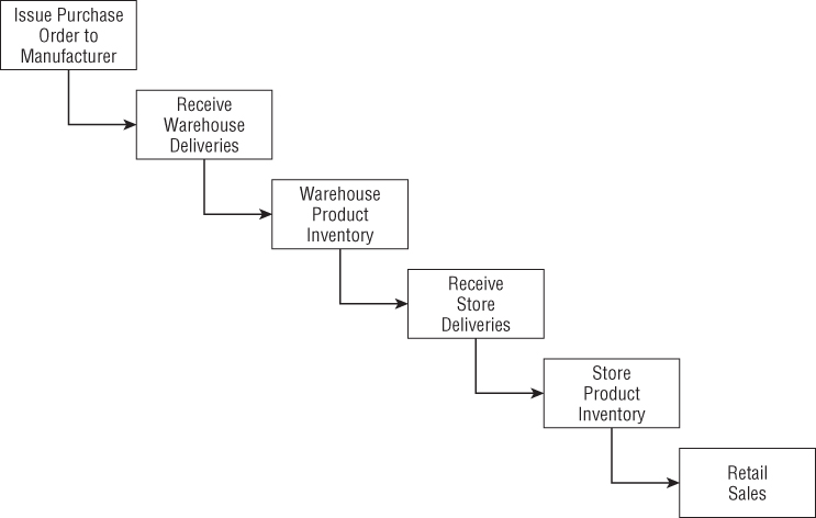
Most organizations have an underlying value chain of key business processes. The value chain identifies the natural, logical flow of an organization's primary activities. For example, a retailer issues purchase orders to product manufacturers. The products are delivered to the retailer's warehouse, where they are held in inventory. A delivery is then made to an individual store, where again the products sit in inventory until a consumer makes a purchase. Figure 4.1 illustrates this subset of a retailer's value chain. Obviously, products sourced from manufacturers that deliver directly to the retail store would bypass the warehousing processes.

Figure 4.1 Subset of a retailer's value chain.

Operational source systems typically produce transactions or snapshots at each step of the value chain. The primary objective of most analytic DW/BI systems is to monitor the performance results of these key processes. Because each process produces unique metrics at unique time intervals with unique granularity and dimensionality, each process typically spawns one or more fact tables. To this end, the value chain provides high-level insight into the overall data architecture for an enterprise DW/BI environment. We'll devote more time to this topic in the “Value Chain Integration” section later in this chapter.

Inventory Models

In the meantime, we'll discuss several complementary inventory models. The first is the inventory periodic snapshot where product inventory levels are measured at regular intervals and placed as separate rows in a fact table. These periodic snapshot rows appear over time as a series of data layers in the dimensional model, much like geologic layers represent the accumulation of sediment over long periods of time. We'll then discuss a second inventory model where every transaction that impacts inventory levels as products move through the warehouse is recorded. Finally, in the third model, we'll describe the inventory accumulating snapshot where a fact table row is inserted for each product delivery and then the row is updated as the product moves through the warehouse. Each model tells a different story. For some analytic requirements, two or even all three models may be appropriate simultaneously.

Inventory Periodic Snapshot

Let's return to our retail case study. Optimized inventory levels in the stores can have a major impact on chain profitability. Making sure the right product is in the right store at the right time minimizes out-of-stocks (where the product isn't available on the shelf to be sold) and reduces overall inventory carrying costs. The retailer wants to analyze daily quantity-on-hand inventory levels by product and store.

It is time to put the four-step dimensional design process to work again. The business process we're interested in analyzing is the periodic snapshotting of retail store inventory. The most atomic level of detail provided by the operational inventory system is a daily inventory for each product in each store. The dimensions immediately fall out of this grain declaration: date, product, and store. This often happens with periodic snapshot fact tables where you cannot express the granularity in the context of a transaction, so a list of dimensions is needed instead. In this case study, there are no additional descriptive dimensions at this granularity. For example, promotion dimensions are typically associated with product movement, such as when the product is ordered, received, or sold, but not with inventory.

The simplest view of inventory involves only a single fact: quantity on hand. This leads to an exceptionally clean dimensional design, as shown in Figure 4.2.

Figure 4.2 Store inventory periodic snapshot schema.

The date dimension table in this case study is identical to the table developed in Chapter 3 for retail store sales. The product and store dimensions may be decorated with additional attributes that would be useful for inventory analysis. For example, the product dimension could be enhanced with columns such as the minimum reorder quantity or the storage requirement, assuming they are constant and discrete descriptors of each product. If the minimum reorder quantity varies for a product by store, it couldn't be included as a product dimension attribute. In the store dimension, you might include attributes to identify the frozen and refrigerated storage square footages.

Even a schema as simple as Figure 4.2 can be very useful. Numerous insights can be derived if inventory levels are measured frequently for many products in many locations. However, this periodic snapshot fact table faces a serious challenge that Chapter 3's sales transaction fact table did not. The sales fact table was reasonably sparse because you don't sell every product in every shopping cart. Inventory, on the other hand, generates dense snapshot tables. Because the retailer strives to avoid out-of-stock situations in which the product is not available, there may be a row in the fact table for every product in every store every day. In that case you would include the zero out-of-stock measurements as explicit rows. For the grocery retailer with 60,000 products stocked in 100 stores, approximately 6 million rows (60,000 products x 100 stores) would be inserted with each nightly fact table load. However, because the row width is just 14 bytes, the fact table would grow by only 84 MB with each load.

Although the data volumes in this case are manageable, the denseness of some periodic snapshots may mandate compromises. Perhaps the most obvious is to reduce the snapshot frequencies over time. It may be acceptable to keep the last 60 days of inventory at the daily level and then revert to less granular weekly snapshots for historical data. In this way, instead of retaining 1,095 snapshots during a 3-year period, the number could be reduced to 208 total snapshots; the 60 daily and 148 weekly snapshots should be stored in two separate fact tables given their unique periodicity.

Semi-Additive Facts

We stressed the importance of fact additivity in Chapter 3. In the inventory snapshot schema, the quantity on hand can be summarized across products or stores and result in a valid total. Inventory levels, however, are not additive across dates because they represent snapshots of a level or balance at one point in time. Because inventory levels (and all forms of financial account balances) are additive across some dimensions but not all, we refer to them as semi-additive facts.

The semi-additive nature of inventory balance facts is even more understandable if you think about your checking account balances. On Monday, presume that you have $50 in your account. On Tuesday, the balance remains unchanged. On Wednesday, you deposit another $50 so the balance is now $100. The account has no further activity through the end of the week. On Friday, you can't merely add up the daily balances during the week and declare that the ending balance is $400 (based on $50 + $50 + $100 + $100 + $100). The most useful way to combine account balances and inventory levels across dates is to average them (resulting in an $80 average balance in the checking example). You are probably familiar with your bank referring to the average daily balance on a monthly account summary.

Unfortunately, you cannot use the SQL AVG function to calculate the average over time. This function averages over all the rows received by the query, not just the number of dates. For example, if a query requested the average inventory for a cluster of three products in four stores across seven dates (e.g., the average daily inventory of a brand in a geographic region during a week), the SQL AVG function would divide the summed inventory value by 84 (3 products × 4 stores × 7 dates). Obviously, the correct answer is to divide the summed inventory value by 7, which is the number of daily time periods.

OLAP products provide the capability to define aggregation rules within the cube, so semi-additive measures like balances are less problematic if the data is deployed via OLAP cubes.

Enhanced Inventory Facts

The simplistic view in the periodic inventory snapshot fact table enables you to see a time series of inventory levels. For most inventory analysis, quantity on hand isn't enough. Quantity on hand needs to be used in conjunction with additional facts to measure the velocity of inventory movement and develop other interesting metrics such as the number of turns and number of days' supply.

If quantity sold (or equivalently, quantity shipped for a warehouse location) was added to each fact row, you could calculate the number of turns and days' supply. For daily inventory snapshots, the number of turns measured each day is calculated as the quantity sold divided by the quantity on hand. For an extended time span, such as a year, the number of turns is the total quantity sold divided by the daily average quantity on hand. The number of days' supply is a similar calculation. Over a time span, the number of days' supply is the final quantity on hand divided by the average quantity sold.

In addition to the quantity sold, inventory analysts are also interested in the extended value of the inventory at cost, as well as the value at the latest selling price. The initial periodic snapshot is embellished in Figure 4.3.

Figure 4.3 Enhanced inventory periodic snapshot.

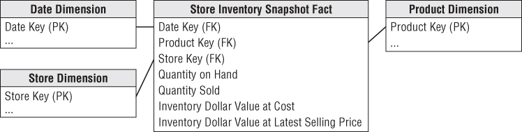
Notice that quantity on hand is semi-additive, but the other measures in the enhanced periodic snapshot are all fully additive. The quantity sold amount has been rolled up to the snapshot's daily granularity. The valuation columns are extended, additive amounts. In some periodic snapshot inventory schemas, it is useful to store the beginning balance, the inventory change or delta, along with the ending balance. In this scenario, the balances are again semi-additive, whereas the deltas are fully additive across all the dimensions.

The periodic snapshot is the most common inventory schema. We'll briefly discuss two alternative perspectives that complement the inventory snapshot just designed. For a change of pace, rather than describing these models in the context of the retail store inventory, we'll move up the value chain to discuss the inventory located in the warehouses.

Inventory Transactions

A second way to model an inventory business process is to record every transaction that affects inventory. Inventory transactions at the warehouse might include the following:

• Receive product.
• Place product into inspection hold.
• Release product from inspection hold.
• Return product to vendor due to inspection failure.
• Place product in bin.
• Pick product from bin.
• Package product for shipment.
• Ship product to customer.
• Receive product from customer.
• Return product to inventory from customer return.
• Remove product from inventory.

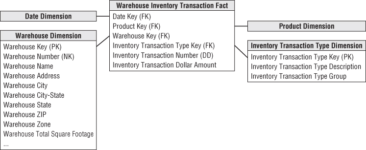
Each inventory transaction identifies the date, product, warehouse, vendor, transaction type, and in most cases, a single amount representing the inventory quantity impact caused by the transaction. Assuming the granularity of the fact table is one row per inventory transaction, the resulting schema is illustrated in Figure 4.4.

Figure 4.4 Warehouse inventory transaction model.

Even though the transaction fact table is simple, it contains detailed information that mirrors individual inventory manipulations. The transaction fact table is useful for measuring the frequency and timing of specific transaction types to answer questions that couldn't be answered by the less granular periodic snapshot.

Even so, it is impractical to use the transaction fact table as the sole basis for analyzing inventory performance. Although it is theoretically possible to reconstruct the exact inventory position at any moment in time by rolling all possible transactions forward from a known inventory position, it is too cumbersome and impractical for broad analytic questions that span dates, products, warehouses, or vendors.

Before leaving the transaction fact table, our example presumes each type of transaction impacting inventory levels positively or negatively has consistent dimensionality: date, product, warehouse, vendor, and transaction type. We recognize some transaction types may have varied dimensionality in the real world. For example, a shipper may be associated with the warehouse receipts and shipments;customer information is likely associated with shipments and customer returns. If the transactions' dimensionality varies by event, then a series of related fact tables should be designed rather than capturing all inventory transactions in a single fact table.

Inventory Accumulating Snapshot

The final inventory model is the accumulating snapshot. Accumulating snapshot fact tables are used for processes that have a definite beginning, definite end, and identifiable milestones in between. In this inventory model, one row is placed in the fact table when a particular product is received at the warehouse. The disposition of the product is tracked on this single fact row until it leaves the warehouse. In this example, the accumulating snapshot model is only possible if you can reliably distinguish products received in one shipment from those received at a later time; it is also appropriate if you track product movement by product serial number or lot number.

Now assume that inventory levels for a product lot captured a series of well-defined events or milestones as it moves through the warehouse, such as receiving, inspection, bin placement, and shipping. As illustrated in Figure 4.5, the inventory accumulating snapshot fact table with its multitude of dates and facts looks quite different from the transaction or periodic snapshot schemas.

Figure 4.5 Warehouse inventory accumulating snapshot.

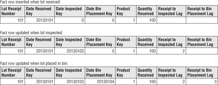
The accumulating snapshot fact table provides an updated status of the lot as it moves through standard milestones represented by multiple date-valued foreign keys. Each accumulating snapshot fact table row is updated repeatedly until the products received in a lot are completely depleted from the warehouse, as shown in Figure 4.6.

Figure 4.6 Evolution of an accumulating snapshot fact row.

Fact Table Types

There are just three fundamental types of fact tables: transaction, periodic snapshot, and accumulating snapshot. Amazingly, this simple pattern holds true regardless of the industry. All three types serve a useful purpose; you often need two complementary fact tables to get a complete picture of the business, yet the administration and rhythm of the three fact tables are quite different. Figure 4.7 compares and contrasts the variations.

Figure 4.7 Fact table type comparisons.

Transaction Fact Tables

The most fundamental view of the business's operations is at the individual transaction or transaction line level. These fact tables represent an event that occurred at an instantaneous point in time. A row exists in the fact table for a given customer or product only if a transaction event occurred. Conversely, a given customer or product likely is linked to multiple rows in the fact table because hopefully the customer or product is involved in more than one transaction.

Transaction data fits easily into a dimensional framework. Atomic transaction data is the most naturally dimensional data, enabling you to analyze behavior in extreme detail. After a transaction has been posted in the fact table, you typically don't revisit it.

Having made a solid case for the charm of transaction detail, you may be thinking that all you need is a big, fast server to handle the gory transaction minutiae, and your job is over. Unfortunately, even with transaction level data, there are business questions that are impractical to answer using only these details. As indicated earlier, you cannot survive on transactions alone.

Periodic Snapshot Fact Tables

Periodic snapshots are needed to see the cumulative performance of the business at regular, predictable time intervals. Unlike the transaction fact table where a row is loaded for each event occurrence, with the periodic snapshot, you take a picture (hence the snapshot terminology) of the activity at the end of a day, week, or month, then another picture at the end of the next period, and so on. The periodic snapshots are stacked consecutively into the fact table. The periodic snapshot fact table often is the only place to easily retrieve a regular, predictable view of longitudinal performance trends.

When transactions equate to little pieces of revenue, you can move easily from individual transactions to a daily snapshot merely by adding up the transactions. In this situation, the periodic snapshot represents an aggregation of the transactional activity that occurred during a time period; you would build the snapshot only if needed for performance reasons. The design of the snapshot table is closely related to the design of its companion transaction table in this case. The fact tables share many dimension tables; the snapshot usually has fewer dimensions overall. Conversely, there are usually more facts in a summarized periodic snapshot table than in a transactional table because any activity that happens during the period is fair game for a metric in a periodic snapshot.

In many businesses, however, transaction details are not easily summarized to present management performance metrics. As you saw in this inventory case study, crawling through the transactions would be extremely time-consuming, plus the logic required to interpret the effect of different kinds of transactions on inventory levels could be horrendously complicated, presuming you even have access to the required historical data. The periodic snapshot again comes to the rescue to provide management with a quick, flexible view of inventory levels. Hopefully, the data for this snapshot schema is sourced directly from an operational system that handles these complex calculations. If not, the ETL system must also implement this complex logic to correctly interpret the impact of each transaction type.

Accumulating Snapshot Fact Tables

Last, but not least, the third type of fact table is the accumulating snapshot. Although perhaps not as common as the other two fact table types, accumulating snapshots can be very insightful. Accumulating snapshots represent processes that have a definite beginning and definite end together with a standard set of intermediate process steps. Accumulating snapshots are most appropriate when business users want to perform workflow or pipeline analysis.

Accumulating snapshots always have multiple date foreign keys, representing the predictable major events or process milestones; sometimes there's an additional date column that indicates when the snapshot row was last updated. As we'll discuss in Chapter 6: Order Management, these dates are each handled by a role-playing date dimension. Because most of these dates are not known when the fact row is first loaded, a default surrogate date key is used for the undefined dates.

Lags Between Milestones and Milestone Counts

Because accumulating snapshots often represent the efficiency and elapsed time of a workflow or pipeline, the fact table typically contains metrics representing the durations or lags between key milestones. It would be difficult to answer duration questions using a transaction fact table because you would need to correlate rows to calculate time lapses. Sometimes the lag metrics are simply the raw difference between the milestone dates or date/time stamps. In other situations, the lag calculation is made more complicated by taking workdays and holidays into consideration.

Accumulating snapshot fact tables sometimes include milestone completion counters, valued as either 0 or 1. Finally, accumulating snapshots often have a foreign key to a status dimension, which is updated to reflect the pipeline's latest status.

Accumulating Snapshot Updates and OLAP Cubes

In sharp contrast to the other fact table types, you purposely revisit accumulating snapshot fact table rows to update them. Unlike the periodic snapshot where the prior snapshots are preserved, the accumulating snapshot merely reflects the most current status and metrics. Accumulating snapshots do not attempt to accommodate complex scenarios that occur infrequently. The analysis of these outliers can always be done with the transaction fact table.

It is worth noting that accumulating snapshots are typically problematic for OLAP cubes. Because updates to an accumulating snapshot force both facts and dimension foreign keys to change, much of the cube would need to be reprocessed with updates to these snapshots, unless the fact row is only loaded once the pipeline occurrence is complete.

Complementary Fact Table Types

Sometimes accumulating and periodic snapshots work in conjunction with one another, such as when you incrementally build the monthly snapshot by adding the effect of each day's transactions to a rolling accumulating snapshot while also storing 36 months of historical data in a periodic snapshot. Ideally, when the last day of the month has been reached, the accumulating snapshot simply becomes the new regular month in the time series, and a new accumulating snapshot is started the next day.

Transactions and snapshots are the yin and yang of dimensional designs. Used together, companion transaction and snapshot fact tables provide a complete view of the business. Both are needed because there is often no simple way to combine these two contrasting perspectives in a single fact table. Although there is some theoretical data redundancy between transaction and snapshot tables, you don't object to such redundancy because as DW/BI publishers, your mission is to publish data so that the organization can effectively analyze it. These separate types of fact tables each provide different vantage points on the same story. Amazingly, these three types of fact tables turn out to be all the fact table types needed for the use cases described in this book.

Value Chain Integration

Now that we've completed the design of three inventory models, let's revisit our earlier discussion about the retailer's value chain. Both business and IT organizations are typically interested in value chain integration. Business management needs to look across the business's processes to better evaluate performance. For example, numerous DW/BI projects have focused on better understanding customer behavior from an end-to-end perspective. Obviously, this requires the ability to consistently look at customer information across processes, such as quotes, orders, invoicing, payments, and customer service. Similarly, organizations want to analyze their products across processes, or their employees, students, vendors, and so on.

IT managers recognize integration is needed to deliver on the promises of data warehousing and business intelligence. Many consider it their fiduciary responsibility to manage the organization's information assets. They know they're not fulfilling their responsibilities if they allow standalone, nonintegrated databases to proliferate. In addition to addressing the business's needs, IT also benefits from integration because it allows the organization to better leverage scarce resources and gain efficiencies through the use of reusable components.

Fortunately, the senior managers who typically are most interested in integration also have the necessary organizational influence and economic willpower to make it happen. If they don't place a high value on integration, you face a much more serious organizational challenge, or put more bluntly, your integration project will probably fail. It shouldn't be the sole responsibility of the DW/BI manager to garner organizational consensus for integration across the value chain. The political support of senior management is important; it takes the DW/BI manager off the hook and places the burden on senior leadership's shoulders where it belongs.

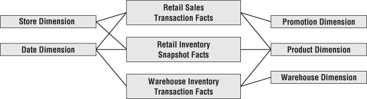
In Chapters 3 and 4, we modeled data from several processes of the retailer's value chain. Although separate fact tables in separate dimensional schemas represent the data from each process, the models share several common business dimensions: date, product, and store. We've logically represented this dimension sharing in Figure 4.8. Using shared, common dimensions is absolutely critical to designing dimensional models that can be integrated.

Figure 4.8 Sharing dimensions among business processes.

Enterprise Data Warehouse Bus Architecture

Obviously, building the enterprise's DW/BI system in one galactic effort is too daunting, yet building it as isolated pieces defeats the overriding goal of consistency. For long-term DW/BI success, you need to use an architected, incremental approach to build the enterprise's warehouse. The approach we advocate is the enterprise data warehouse bus architecture.

Understanding the Bus Architecture

Contrary to popular belief, the word bus is not shorthand for business; it's an old term from the electrical power industry that is now used in the computer industry. A bus is a common structure to which everything connects and from which everything derives power. The bus in a computer is a standard interface specification that enables you to plug in a disk drive, DVD, or any number of other specialized cards or devices. Because of the computer's bus standard, these peripheral devices work together and usefully coexist, even though they were manufactured at different times by different vendors.

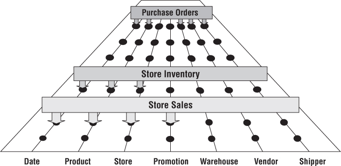
If you refer back to the value chain diagram in Figure 4.1, you can envision many business processes plugging into the enterprise data warehouse bus, as illustrated in Figure 4.9. Ultimately, all the processes of an organization's value chain create a family of dimensional models that share a comprehensive set of common, conformed dimensions.

Figure 4.9 Enterprise data warehouse bus with shared dimensions.

The enterprise data warehouse bus architecture provides a rational approach to decomposing the enterprise DW/BI planning task. The master suite of standardized dimensions and facts has a uniform interpretation across the enterprise. This establishes the data architecture framework. You can then tackle the implementation of separate process-centric dimensional models, with each implementation closely adhering to the architecture. As the separate dimensional models become available, they fit together like the pieces of a puzzle. At some point, enough dimensional models exist to make good on the promise of an integrated enterprise DW/BI environment.

The bus architecture enables DW/BI managers to get the best of both worlds. They have an architectural framework guiding the overall design, but the problem has been divided into bite-sized business process chunks that can be implemented in realistic time frames. Separate development teams follow the architecture while working fairly independently and asynchronously.

The bus architecture is independent of technology and database platforms. All flavors of relational and OLAP-based dimensional models can be full participants in the enterprise data warehouse bus if they are designed around conformed dimensions and facts. DW/BI systems inevitably consist of separate machines with different operating systems and database management systems. Designed coherently, they share a common architecture of conformed dimensions and facts, allowing them to be fused into an integrated whole.

Enterprise Data Warehouse Bus Matrix

We recommend using an enterprise data warehouse bus matrix to document and communicate the bus architecture, as illustrated in Figure 4.10. Others have renamed the bus matrix, such as the conformance or event matrix, but these are merely synonyms for this fundamental Kimball concept first introduced in the 1990s.

Figure 4.10 Sample enterprise data warehouse bus matrix for a retailer.

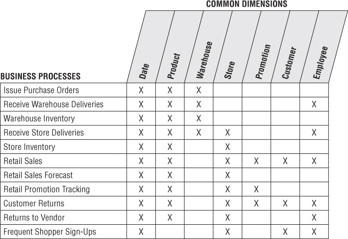
Working in a tabular fashion, the organization's business processes are represented as matrix rows. It is important to remember you are identifying business processes, not the organization's business departments. The matrix rows translate into dimensional models representing the organization's primary activities and events, which are often recognizable by their operational source. When it's time to tackle a DW/BI development project, start with a single business process matrix row because that minimizes the risk of signing up for an overly ambitious implementation. Most implementation risk comes from biting off too much ETL system design and development. Focusing on the results of a single process, often captured by a single underlying source system, reduces the ETL development risk.

After individual business processes are enumerated, you sometimes identify more complex consolidated processes. Although dimensional models that cross processes can be immensely beneficial in terms of both query performance and ease of use, they are typically more difficult to implement because the ETL effort grows with each additional major source integrated into a single dimensional model. It is prudent to focus on the individual processes as building blocks before tackling the task of consolidating. Profitability is a classic example of a consolidated process in which separate revenue and cost factors are combined from different processes to provide a complete view of profitability. Although a granular profitability dimensional model is exciting, it is definitely not the first dimensional model you should attempt to implement; you could easily drown while trying to wrangle all the revenue and cost components.

The columns of the bus matrix represent the common dimensions used across the enterprise. It is often helpful to create a list of core dimensions before filling in the matrix to assess whether a given dimension should be associated with a business process. The number of bus matrix rows and columns varies by organization. For many, the matrix is surprisingly square with approximately 25 to 50 rows and a comparable number of columns. In other industries, like insurance, there tend to be more columns than rows.

After the core processes and dimensions are identified, you shade or “X” the matrix cells to indicate which columns are related to each row. Presto! You can immediately see the logical relationships and interplay between the organization's conformed dimensions and key business processes.

Multiple Matrix Uses

Creating the enterprise data warehouse bus matrix is one of the most important DW/BI implementation deliverables. It is a hybrid resource that serves multiple purposes, including architecture planning, database design, data governance coordination, project estimating, and organizational communication.

Although it is relatively straightforward to lay out the rows and columns, the enterprise bus matrix defines the overall data architecture for the DW/BI system. The matrix delivers the big picture perspective, regardless of database or technology preferences.

The matrix's columns address the demands of master data management and data integration head-on. As core dimensions participating in multiple dimensional models are defined by folks with data governance responsibilities and built by the DW/BI team, you can envision their use across processes rather than designing in a vacuum based on the needs of a single process, or even worse, a single department. Shared dimensions supply potent integration glue, allowing the business to drill across processes.

Each business process-centric implementation project incrementally builds out the overall architecture. Multiple development teams can work on components of the matrix independently and asynchronously, with confidence they'll fit together. Project managers can look across the process rows to see the dimensionality of each dimensional model at a glance. This vantage point is useful as they're gauging the magnitude of the project's effort. A project focused on a business process with fewer dimensions usually requires less effort, especially if the politically charged dimensions are already sitting on the shelf.

The matrix enables you to communicate effectively within and across data governance and DW/BI teams. Even more important, you can use the matrix to communicate upward and outward throughout the organization. The matrix is a succinct deliverable that visually conveys the master plan. IT management needs to understand this perspective to coordinate across project teams and resist the organizational urge to deploy more departmental solutions quickly. IT management must also ensure that distributed DW/BI development teams are committed to the bus architecture. Business management needs to also appreciate the holistic plan; you want them to understand the staging of the DW/BI rollout by business process. In addition, the matrix illustrates the importance of identifying experts from the business to serve as data governance leaders for the common dimensions. It is a tribute to its simplicity that the matrix can be used effectively to communicate with developers, architects, modelers, and project managers, as well as senior IT and business management.

Opportunity/Stakeholder Matrix

You can draft a different matrix that leverages the same business process rows, but replaces the dimension columns with business functions, such as merchandising, marketing, store operations, and finance. Based on each function's requirements, the matrix cells are shaded to indicate which business functions are interested in which business processes (and projects), as illustrated in Figure 4.11's opportunity/stakeholder matrix variation. It also identifies which groups need to be invited to the detailed requirements, dimensional modeling, and BI application specification parties after a process-centric row is queued up as a project.

Figure 4.11 Opportunity/stakeholder matrix.

Common Bus Matrix Mistakes

When drafting a bus matrix, people sometimes struggle with the level of detail expressed by each row, resulting in the following missteps:

• Departmental or overly encompassing rows. The matrix rows shouldn't correspond to the boxes on a corporate organization chart representing functional groups. Some departments may be responsible or acutely interested in a single business process, but the matrix rows shouldn't look like a list of the CEO's direct reports.
• Report-centric or too narrowly defined rows. At the opposite extreme, the bus matrix shouldn't resemble a laundry list of requested reports. A single business process supports numerous analyses; the matrix row should reference the business process, not the derivative reports or analytics.

When defining the matrix columns, architects naturally fall into the similar traps of defining columns that are either too broad or too narrow:

• Overly generalized columns. A “person” column on the bus matrix may refer to a wide variety of people, from internal employees to external suppliers and customer contacts. Because there's virtually zero overlap between these populations, it adds confusion to lump them into a single, generic dimension. Similarly, it's not beneficial to put internal and external addresses referring to corporate facilities, employee addresses, and customer sites into a generic location column in the matrix.
• Separate columns for each level of a hierarchy. The columns of the bus matrix should refer to dimensions at their most granular level. Some business process rows may require an aggregated version of the detailed dimension, such as inventory snapshot metrics at the weekly level. Rather than creating separate matrix columns for each level of the calendar hierarchy, use a single column for dates. To express levels of detail above a daily grain, you can denote the granularity within the matrix cell; alternatively, you can subdivide the date column to indicate the hierarchical level associated with each business process row. It's important to retain the overarching identification of common dimensions deployed at different levels of granularity. Some industry pundits advocate matrices that treat every dimension table attribute as a separate, independent column; this defeats the concept of dimensions and results in a completely unruly matrix.

Retrofitting Existing Models to a Bus Matrix

It is unacceptable to build separate dimensional models that ignore a framework tying them together. Isolated, independent dimensional models are worse than simply a lost opportunity for analysis. They deliver access to irreconcilable views of the organization and further enshrine the reports that cannot be compared with one another. Independent dimensional models become legacy implementations in their own right; by their existence, they block the development of a coherent DW/BI environment.

So what happens if you're not starting with a blank slate? Perhaps several dimensional models have been constructed without regard to an architecture using conformed dimensions. Can you rescue your stovepipes and convert them to the bus architecture? To answer this question, you should start first with an honest appraisal of your existing non-integrated dimensional structures. This typically entails meetings with the separate teams (including the clandestine pseudo IT teams within business organizations) to determine the gap between the current environment and the organization's architected goal. When the gap is understood, you need to develop an incremental plan to convert the standalone dimensional models to the enterprise architecture. The plan needs to be internally sold. Senior IT and business management must understand the current state of data chaos, the risks of doing nothing, and the benefits of moving forward according to your game plan. Management also needs to appreciate that the conversion will require a significant commitment of support, resources, and funding.

If an existing dimensional model is based on a sound dimensional design, perhaps you can map an existing dimension to a standardized version. The original dimension table would be rebuilt using a cross-reference map. Likewise, the fact table would need to be reprocessed to replace the original dimension keys with the conformed dimension keys. Of course, if the original and conformed dimension tables contain different attributes, rework of the preexisting BI applications and queries is inevitable.

More typically, existing dimensional models are riddled with dimensional modeling errors beyond the lack of adherence to standardized dimensions. In some cases, the stovepipe dimensional model has outlived its useful life. Isolated dimensional models often are built for a specific functional area. When others try to leverage the data, they typically discover that the dimensional model was implemented at an inappropriate level of granularity and is missing key dimensionality. The effort required to retrofit these dimensional models into the enterprise DW/BI architecture may exceed the effort to start over from scratch. As difficult as it is to admit, stovepipe dimensional models often have to be shut down and rebuilt in the proper bus architecture framework.

Conformed Dimensions

Now that you understand the importance of the enterprise bus architecture, let's further explore the standardized conformed dimensions that serve as the cornerstone of the bus because they're shared across business process fact tables. Conformed dimensions go by many other aliases: common dimensions, master dimensions, reference dimensions, and shared dimensions. Conformed dimensions should be built once in the ETL system and then replicated either logically or physically throughout the enterprise DW/BI environment. When built, it's extremely important that the DW/BI development teams take the pledge to use these dimensions. It's a policy decision that is critical to making the enterprise DW/BI system function; their usage should be mandated by the organization's CIO.

Drilling Across Fact Tables

In addition to consistency and reusability, conformed dimensions enable you to combine performance measurements from different business processes in a single report, as illustrated in Figure 4.12. You can use multipass SQL to query each dimensional model separately and then outer-join the query results based on a common dimension attribute, such as Figure 4.12's product name. The full outer-join ensures all rows are included in the combined report, even if they only appear in one set of query results. This linkage, often referred to as drill across, is straightforward if the dimension table attribute values are identical.

Figure 4.12 Drilling across fact tables with conformed dimension attributes.

Drilling across is supported by many BI products and platforms. Their implementations differ on whether the results are joined in temporary tables, the application server, or the report. The vendors also use different terms to describe this technique, including multipass, multi-select, multi-fact, or stitch queries. Because metrics from different fact tables are brought together with a drill-across query, often any cross-fact calculations must be done in the BI application after the separate conformed results have been returned.

Conformed dimensions come in several different flavors, as described in the following sections.

Identical Conformed Dimensions

At the most basic level, conformed dimensions mean the same thing with every possible fact table to which they are joined. The date dimension table connected to the sales facts is identical to the date dimension table connected to the inventory facts. Identical conformed dimensions have consistent dimension keys, attribute column names, attribute definitions, and attribute values (which translate into consistent report labels and groupings). Dimension attributes don't conform if they're called Month in one dimension and Month Name in another; likewise, they don't conform if the attribute value is “July” in one dimension and “JULY” in another. Identical conformed dimensions in two dimensional models may be the same physical table within the database. However, given the typical complexity of the DW/BI system's technical environment with multiple database platforms, it is more likely that the dimension is built once in the ETL system and then duplicated synchronously outward to each dimensional model. In either case, the conformed date dimensions in both dimensional models have the same number of rows, same key values, same attribute labels, same attribute data definitions, and same attribute values. Attribute column names should be uniquely labeled across dimensions.

Most conformed dimensions are defined naturally at the most granular level possible. The product dimension's grain will be the individual product; the date dimension's grain will be the individual day. However, sometimes dimensions at the same level of granularity do not fully conform. For example, there might be product and store attributes needed for inventory analysis, but they aren't appropriate for analyzing retail sales data. The dimension tables still conform if the keys and common columns are identical, but the supplemental attributes used by the inventory schema are not conformed. It is physically impossible to drill across processes using these add-on attributes.

Shrunken Rollup Conformed Dimension with Attribute Subset

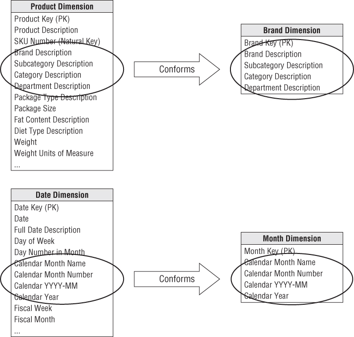
Dimensions also conform when they contain a subset of attributes from a more granular dimension. Shrunken rollup dimensions are required when a fact table captures performance metrics at a higher level of granularity than the atomic base dimension. This would be the case if you had a weekly inventory snapshot in addition to the daily snapshot. In other situations, facts are generated by another business process at a higher level of granularity. For example, the retail sales process captures data at the atomic product level, whereas forecasting generates data at the brand level. You couldn't share a single product dimension table across the two business process schemas because the granularity is different. The product and brand dimensions still conform if the brand table attributes are a strict subset of the atomic product table's attributes. Attributes that are common to both the detailed and rolled-up dimension tables, such as the brand and category descriptions, should be labeled, defined, and identically valued in both tables, as illustrated in Figure 4.13. However, the primary keys of the detailed and rollup dimension tables are separate.

Figure 4.13 Conforming shrunken rollup dimensions.

Shrunken Conformed Dimension with Row Subset

Another case of conformed dimension subsetting occurs when two dimensions are at the same level of detail, but one represents only a subset of rows. For example, a corporate product dimension contains rows for the full portfolio of products across multiple disparate lines of business, as illustrated in Figure 4.14. Analysts in the separate businesses may want to view only their subset of the corporate dimension, restricted to the product rows for their business. By using a subset of rows, they aren't encumbered with the corporation's entire product set. Of course, the fact table joined to this subsetted dimension must be limited to the same subset of products. If a user attempts to use a shrunken subset dimension while accessing a fact table consisting of the complete product set, they may encounter unexpected query results because referential integrity would be violated. You need to be cognizant of the potential opportunity for user confusion or error with dimension row subsetting. We will further elaborate on dimension subsets when we discuss supertype and subtype dimensions in Chapter 10: Financial Services.

Figure 4.14 Conforming dimension subsets at the same granularity.

Conformed date and month dimensions are a unique example of both rowand column dimension subsetting. Obviously, you can't simply use the same date dimension table for daily and monthly fact tables because of the difference in rollup granularity. However, the month dimension may consist of the month-end daily date table rows with the exclusion of all columns that don't apply at the monthly granularity, such as the weekday/weekend indicator, week ending date, holiday indicator, day number within year, and others. Sometimes a month-end indicator on the daily date dimension is used to facilitate creation of this month dimension table.

Shrunken Conformed Dimensions on the Bus Matrix

The bus matrix identifies the reuse of common dimensions across business processes.Typically, the shaded cells of the matrix indicate that the atomic dimension is associated with a given process. When shrunken rollup or subset dimensions are involved, you want to reinforce their conformance with the atomic dimensions. Therefore, you don't want to create a new, unrelated column on the bus matrix. Instead, there are two viable approaches to represent the shrunken dimensions within the matrix, as illustrated in Figure 4.15:

• Mark the cell for the atomic dimension, but then textually document the rollup or row subset granularity within the cell.
• Subdivide the dimension column to indicate the common rollup or subset granularities, such as day and month if processes collect data at both of these grains.

Figure 4.15 Alternatives for identifying shrunken dimensions on the bus matrix.

Limited Conformity

Now that we've preached about the importance of conformed dimensions, we'll discuss the situation in which it may not be realistic or necessary to establish conformed dimensions for the organization. If a conglomerate has subsidiaries spanning widely varied industries, there may be little point in trying to integrate. If each line of business has unique customers and unique products and there's no interest in cross-selling across lines, it may not make sense to attempt an enterprise architecture because there likely isn't much perceived business value. The willingness to seek a common definition for product, customer, or other core dimensions is a major litmus test for an organization theoretically intent on building an enterprise DW/BI system. If the organization is unwilling to agree on common definitions, the organization shouldn't attempt to build an enterprise DW/BI environment. It would be better to build separate, self-contained data warehouses for each subsidiary. But then don't complain when someone asks for “enterprise performance” without going through this logic.

Although organizations may find it difficult to combine data across disparate lines of business, some degree of integration is typically an ultimate goal. Rather than throwing your hands in the air and declaring it can't possibly be done, you should start down the path toward conformity. Perhaps there are a handful of attributes that can be conformed across lines of business. Even if it is merely a product description, category, and line of business attribute that is common to all businesses, this least-common-denominator approach is still a step in the right direction. You don't need to get everyone to agree on everything related to a dimension before proceeding.

Importance of Data Governance and Stewardship

We've touted the importance of conformed dimensions, but we also need to acknowledge a key challenge: reaching enterprise consensus on dimension attribute names and contents (and the handling of content changes which we'll discuss in Chapter 5: Procurement). In many organizations, business rules and data definitions have traditionally been established departmentally. The consequences of this commonly encountered lack of data governance and control are the ubiquitous departmental data silos that perpetuate similar but slightly different versions of the truth. Business and IT management need to recognize the importance of addressing this shortfall if you stand any chance of bringing order to the chaos; if management is reluctant to drive change, the project will never achieve its goals.

Once the data governance issues and opportunities are acknowledged by senior leadership, resources need to be identified to spearhead the effort. IT is often tempted to try leading the charge. They are frustrated by the isolated projects re-creating data around the organization, consuming countless IT and outside resources while delivering inconsistent solutions that ultimately just increase the complexity of the organization's data architecture at significant cost. Although IT can facilitate the definition of conformed dimensions, it is seldom successful as the sole driver, even if it's a temporary assignment. IT simply lacks the organizational authority to make things happen.

Business-Driven Governance

To boost the likelihood of business acceptance, subject matter experts from the business need to lead the initiative. Leading a cross-organizational governance program is not for the faint of heart. The governance resources identified by business leadership should have the following characteristics:

• Respect from the organization
• Broad knowledge of the enterprise's operations
• Ability to balance organizational needs against departmental requirements
• Gravitas and authority to challenge the status quo and enforce policies
• Strong communication skills
• Politically savvy negotiation and consensus building skills

Clearly, not everyone is cut out for the job! Typically those tapped to spearhead the governance program are highly valued and in demand. It takes the right skills, experience, and confidence to rationalize diverse business perspectives and drive the design of common reference data, together with the necessary organizational compromises. Over the years, some have criticized conformed dimensions as being too hard. Yes, it's difficult to get people in different corners of the business to agree on common attribute names, definitions, and values, but that's the crux of unified, integrated data. If everyone demands their own labels and business rules, there's no chance of delivering on the promises made to establish a single version of the truth. The data governance program is critical in facilitating a culture shift away from the typical siloed environment in which each department retains control of their data and analytics to one where information is shared and leveraged across the organization.

Governance Objectives

One of the key objectives of the data governance function is to reach agreement on data definitions, labels, and domain values so that everyone is speaking the same language. Otherwise, the same words may describe different things; different words may describe the same thing; and the same value may have different meaning. Establishing common master data is often a politically charged issue; the challenges are cultural and geopolitical rather than technical. Defining a foundation of master descriptive conformed dimensions requires effort. But after it's agreed upon, subsequent DW/BI efforts can leverage the work, both ensuring consistency and reducing the implementation's delivery cycle time.

In addition to tackling data definitions and contents, the data governance function also establishes policies and responsibilities for data quality and accuracy, as well as data security and access controls.

Historically, DW/BI teams created the “recipes” for conformed dimensions and managed the data cleansing and integration mapping in the ETL system; the operational systems focused on accurately capturing performance metrics, but there was often little effort to ensure consistent common reference data. Enterprise resource planning (ERP) systems promised to fill the void, but many organizations still rely on separate best-of-breed point solutions for niche requirements. Recently, operational master data management (MDM) solutions have addressed the need for centralized master data at the source where the transactions are captured. Although technology can encourage data integration, it doesn't fix the problem. A strong data governance function is a necessary prerequisite for conforming information regardless of technical approach.

Conformed Dimensions and the Agile Movement

Some lament that although they want to deliver and share consistently defined master conformed dimensions in their DW/BI environments, it's “just not feasible.” They explain they would if they could, but with senior management focused on using agile development techniques, it's “impossible” to take the time to get organizational agreement on conformed dimensions. You can turn this argument upside down by challenging that conformed dimensions enable agile DW/BI development, along with agile decision making.

Conformed dimensions allow a dimension table to be built and maintained once rather than re-creating slightly different versions during each development cycle. Reusing conformed dimensions across projects is where you get the leverage for more agile DW/BI development. As you flesh out the portfolio of master conformed dimensions, the development crank starts turning faster and faster. The time-to-market for a new business process data source shrinks as developers reuse existing conformed dimensions. Ultimately, new ETL development focuses almost exclusively on delivering more fact tables because the associated dimension tables are already sitting on the shelf ready to go.

Defining a conformed dimension requires organizational consensus and commitment to data stewardship. But you don't need to get everyone to agree on every attribute in every dimension table. At a minimum, you should identify a subset of attributes that have significance across the enterprise. These commonly referenced descriptive characteristics become the starter set of conformed attributes, enabling drill-across integration. Even just a single attribute, such as enterprise product category, is a viable starting point for the integration effort. Over time, you can iteratively expand from this minimalist starting point by adding attributes. These dimensions could be tackled during architectural agile sprints. When a series of sprint deliverables combine to deliver sufficient value, they constitute a release to the business users.

If you fail to focus on conformed dimensions because you're under pressure to deliver something yesterday, the departmental analytic data silos will likely have inconsistent categorizations and labels. Even more troubling, data sets may look like they can be compared and integrated due to similar labels, but the underlying business rules may be slightly different. Business users waste inordinate amounts of time trying to reconcile and resolve these data inconsistencies, which negatively impact their ability to be agile decision makers.

The senior IT managers who are demanding agile systems development practices should be exerting even greater organizational pressure, in conjunction with their peers in the business, on the development of consistent conformed dimensions if they're interested in both long-term development efficiencies and long-term decision-making effectiveness across the enterprise.

Conformed Facts

Thus far we have considered the central task of setting up conformed dimensions to tie dimensional models together. This is 95 percent or more of the data architecture effort. The remaining 5 percent of the effort goes into establishing conformed fact definitions.

Revenue, profit, standard prices and costs, measures of quality and customer satisfaction, and other key performance indicators (KPIs) are facts that must also conform. If facts live in more than one dimensional model, the underlying definitions and equations for these facts must be the same if they are to be called the same thing. If they are labeled identically, they need to be defined in the same dimensional context and with the same units of measure from dimensional model to dimensional model. For example, if several business processes report revenue, then these separate revenue metrics can be added and compared only if they have the same financial definitions. If there are definitional differences, then it is essential that the revenue facts be labeled uniquely.

Sometimes a fact has a natural unit of measure in one fact table and another natural unit of measure in another fact table. For example, the flow of product down the retail value chain may best be measured in shipping cases at the warehouse but in scanned units at the store. Even if all the dimensional considerations have been correctly taken into account, it would be difficult to use these two incompatible units of measure in one drill-across report. The usual solution to this kind of problem is to refer the user to a conversion factor buried in the product dimension table and hope that the user can find the conversion factor and correctly use it. This is unacceptable for both overhead and vulnerability to error. The correct solution is to carry the fact in both units of measure, so a report can easily glide down the value chain, picking off comparable facts. Chapter 6: Order Management talks more about multiple units of measure.

Summary

In this chapter we developed dimensional models for the three complementary views of inventory. The periodic snapshot is a good choice for long-running, continuously replenished inventory scenarios. The accumulating snapshot is a good choice for finite inventory pipeline situations with a definite beginning and end. Finally, most inventory analysis will require a transactional schema to augment these snapshot models.

We introduced key concepts surrounding the enterprise data warehouse bus architecture and matrix. Each business process of the value chain, supported by a primary source system, translates into a row in the bus matrix, and eventually, a dimensional model. The matrix rows share a surprising number of standardized, conformed dimensions. Developing and adhering to the enterprise bus architecture is an absolute must if you intend to build a DW/BI system composed of an integrated set of dimensional models.