
5. Adding Capacity to the Model
In the previous models, we did not consider capacity. Each facility could be as large as it needed to be to service the demand assigned to it. This may not always be a good assumption. In this chapter, we want to consider how capacity impacts our network design models.
Even though every facility in a supply chain has capacity limitations, you often do not need to include those limitations in the model. The main reason to omit capacity from your model is that it doesn’t impact the decision you are trying to make. The following are reasons that capacity may not impact your decision.
First, when you ask the model to open multiple facilities, it will naturally tend to balance the demand across the facilities to minimize average distance or cost.
Second, especially for warehouses, increasing capacity can be relatively inexpensive. With warehouses, you may be using a third-party warehouse and extra space simply means asking for it. Even when you are not using a third party, many warehouses can easily expand in space. For manufacturing sites, extra capacity may simply mean hiring more workers (which you would have to do anywhere in the supply chain). Of course, the exception to both of these cases is when you have highly automated facilities with expensive equipment.
Third, often the decisions you are making concern the long term. And, in that case, today’s capacity is not fixed for the future. You want the model to return the size of the facility needed. You do not want to fix this beforehand.
However, there are instances when capacity will be critical to your network design study. For example, if you are making decisions about investing in expensive, highly automated plants or warehouses, or are deciding where to place a specialized production line, or trying to determine how many shifts you want a plant to operate.
Following are some short cases that help highlight some issues you may find when modeling capacity.
Case Study: Swimming Pool Chemicals
We worked with a company that made and sold chemicals for swimming pools. Because they could never exactly predict where and when the first warm weekend would hit and everyone would want to buy supplies for their swimming pools, they wanted to position their product in warehouses that were as close to the customers as possible. However, they also wanted to minimize the number of warehouses so that they had some flexibility. For example, if they ship product to a region and that region does not get warm weather, they may have to ship this product out to another warehouse. They did not have the luxury of being able to afford these extra shipments. So they wanted to avoid it, if possible.
However, they had one other thing to consider: Their products were labeled as hazardous, and if the warehouse where they were being stored caught fire, the fire would be difficult to contain and would strain the local firefighting squads. Therefore, the local fire departments would not allow them to have more than 100,000 units of product in the warehouse.
So when the company designed their supply chain, they had to consider this capacity constraint. This could change their answer. For example, without capacity constraints it might be best to locate very large facilities near densely populated areas and smaller facilities in other locations. But with this constraint there will tend to be many warehouses at or near the limit of 100,000 units. And, some densely populated markets may have multiple warehouses whereas without the constraint one large warehouse would have been better.
Case Study: Warehouse Capacity Utilization
Sometimes, the use of math in business is not as precise as the use of math in engineering.
When an engineer expresses the capacity of a warehouse, it is the maximum amount of product that can be stored or processed. Here we are talking about the true maximum amount of capacity. Beyond this point, the firm has to rent extra space or take some other measure. At most, a warehouse can be at 100% of capacity. This percentage is the utilization of the warehouse.
We have been involved in many discussions with managers of warehousing or directors of the supply chain where we have heard a quote like this: “Our current utilization of warehouse A is 125% and warehouse B is 133%.” And the manager will stick to these numbers even after you qualify that he is not measuring against some theoretical capacity or a desired level of capacity.
If you are thinking like an engineer, a statement like this can hurt your brain. How can they be running the warehouse at more than capacity? It turns out that warehouse capacity is very hard to measure, and it may not even be possible to come up with a single number that captures it.
Warehouses have three primary functions. They receive product, they ship product, and they store product.
The capacity for shipping and receiving depends on how many shifts you run, how many people or resources (like automated pickers) you have, what kind of equipment you have, and how much space you have dedicated to these functions. In highly automated systems, it may be easier to measure this capacity. In manual systems, you can easily add more people. But as you add people, you increase the congestion in the warehouse and that may lead to less productivity.
The storage capacity is measured by how much physical space you have and how much is in the warehouse at any given time. However, this is not easy to measure. For example, a warehouse may have storage areas where items (mostly in pallets) sit on the floor and areas where items are stored on racks. These warehouses need to leave room for aisles so that you can get to the product. Also, the managers of these warehouses might like to put the same products in the same location so that they can find them. You can understand the difficulty in measuring capacity when the warehouse starts to get full. Most warehouse managers can get creative when they start to run out of space. They can stack items (by stacking pallets or adding racks to the floor storage areas), place the same product in different locations, use the aisles, and not unload incoming trailers (a common trick).
So a warehouse capacity utilization of over 100% is not violating some rule of mathematics. Instead, from a business point of view, it means that the warehouse is very busy. We don’t know whether it is so busy that it is inefficient or whether something should be done about it. That is left for further analysis.
These cases do, however, cause you to pause when modeling warehouse capacity. If a warehouse can handle 120% of capacity, you might not want the model to make different decisions when it hits 100%. Maybe you should include some slack in your measure of flexibility. We’ll have more on this topic later.
Case Study: Paint Company and Capacity
Manufacturing capacity is typically more straightforward to measure than warehousing capacity. And it is usually more expensive to add. Of course, there are some difficulties because the product mix may not be known in advance, the number of setups can impact capacity, and there are always unanticipated problems on the shop floor.
However, these problems can usually be accounted for in network design without too much effort. For our purposes in locating facilities, we can determine how much product can be produced over the year for a given number of shifts. This measure takes into account the product mix (by directly accounting for capacity needed per product), the average amount of time lost to setups, and the average uptime on the lines.
In some cases, hitting a capacity constraint can have serious implications for the business. We worked with a regional U.S. paint company that had two plants—one on the East Coast south of New York City and another in the Southeast near Charlotte, North Carolina. They sold through their own retail stores in about 30 major metro areas east of the Mississippi.
When we first started working with the company, they distributed their product directly from warehouses that were attached to their plants. Because each plant did not make the full assortment of products, they had to ship a lot of product between the two plants so that they could ship a full assortment to their stores.
Paint is very expensive to ship, and they were always looking for ways to reduce transportation costs. So, for example, they considered the following questions:
• Which warehouse should serve which metro area to reduce transfer of paint between the two plant warehouses?
• Should they add a warehouse or two to get closer to their stores and minimize the shipments between the two plant warehouses?
It turned out that a new warehouse to serve the metro areas around Chicago and Minneapolis could reduce transportation costs. However, the company recognized that they also had to design their supply chain for their future growth. Both of their plants were running close to capacity. If they continued to grow at the current rate, they would have to expand one or both of their plants.
By adding future demand to the model and not allowing any expansion, they let the model make a key decision: which markets they should exit. As a result of the analysis, they sold their stores in the Chicago and Minneapolis areas to another paint company, delayed a significant investment in their plant capacity, and reduced their per-unit transportation costs because they were much closer to their demand.
This case clearly highlights the trade-offs when you bump up against true capacity constraints—either you have to add capacity or you have to not meet all your demand. Network modeling can help you make decisions like this.
Adding Capacity to the Model
The previous cases highlight how capacity can play a role in your model and the care you should exercise when adding capacity to your models.
For example, when modeling warehouse capacity, you have to understand whether the capacity measure is a hard constraint or whether there is some slack in the calculation. If there is some slack, adding capacity to the model may mean simply increasing the number you were given to better reflect reality. In other cases, managers will recognize that they cannot really run a facility at 100% capacity. Instead, they want to say that the limit is 80%. You should note that this does not solve our problem of whether this is a hard constraint. Is the 80% the hard constraint or is the 100%?
If the warehouse constraint is real, you need to consider the cost of new warehouse space. If you are using third-party space, adding capacity may just incur extra variable costs. Or if your warehouse systems are relatively simple and manual, adding space may be no problem at all. For example, if you are currently storing product directly on the floor and your ceilings are high enough, you may simply need to add racks to increase the storage capacity. If you need to have a high-speed, highly automated warehouse, you will need to think about a more significant capital investment.
If the warehouse constraint is not in space, but in terms of its ability to process inbound and outbound shipments, increasing capacity may require additional shifts, additional dock doors, or more automation.
With plants, capacity expansion typically comes in three forms:
1. Adding Labor—Extra labor can provide the ability to produce more. Sometimes extra labor can be added in small increments (1 person at a time, for example) or in larger batches (you need to bring in another full crew).
2. Adding Shifts—When you add shifts, you may incur additional fixed costs (to staff up the line, to manage it, and it may be difficult to remove later), as well as additional variable costs.
3. Adding Equipment—This can include anything from investing in the existing equipment to make it faster, to adding production lines, to building a completely new plant.
With both plant and warehouse capacity, you may also need to factor in the time period for capacity. For example, in annual or long-term models, you will model the effective capacity over the year. If you have a very seasonal business, you can adjust the capacity to reflect that fact. For example, you can set your warehouses to average capacity or peak capacity, and you can do the same for plants.
Mathematical Formulation
Initially, we will add only constraints to warehouse capacity. We will assume unbounded production capacity in the model we formulate next.
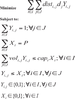
This is identical to the “distance only” problem we formulated in Chapter 3, “Locating Facilities Using a Distance-Based Approach,” with the following changes:
• We create the term capi to measure the capacity of warehouse i. For our purposes here, we have a single measure of capacity and just on the warehouses. This will serve our purposes here of giving you the intuition needed for thinking about capacity. In practice, we model capacity in many ways. At a warehouse we measure it as a storage capacity, a total throughput capacity, or an ability to process inbound or outbound shipments. At a plant, likewise, we can measure capacity by the overall time available in regular time and overtime, the overall tons or units that can be produced, or the maximum amount of a product you can produce. There are many ways to capture capacity at a plant, but because this is effectively the same as for a warehouse, we won’t cover it here.
• We create the term voli,j to measure the effective volume of demand for customer j being assigned to warehouse i. Note that we index this term by both the customer and the warehouse. This allows us to model the possibility that different warehouses might use different units of measurement to determine their capacity, or that different products might be cross-docked with higher levels of efficiency at some facilities. When this term applies to a plant, it has the same definition: It is the amount of a plant’s capacity that is consumed by that customer’s demand. Again, a more detailed version can allow for the capacity consumed to vary with the product as well.
• We add the constraint ![]() which we apply to all warehouses.
which we apply to all warehouses.
This constraint ensures that a warehouse is never assigned more demand than it can handle. Note that if the warehouse capacity is not infinite, this constraint also will ensure that if a customer is assigned to a warehouse, that warehouse must be opened. However, we will not discard the family of Yi,j ≤ Xi constraints, as experience has shown that their inclusion can significantly improve the runtime of our models. (The engineering of optimization problems often involves applying potentially redundant constraints in order to generate efficient runtimes. This phenomenon is but one such argument in favor of purchasing off-the-shelf optimization applications for specific problems, as opposed to using generic tools to create optimization problems by hand.)
Possible Difficulty with Models That Have Capacity Constraints
Like our service-level constraints in the previous chapter, we need now to be careful that the problem is still feasible. That is, it is again possible to create a model such that it is impossible to solve. For example, we can specify 100 units of demand and only 80 units of capacity. In this case, the constraint that we must meet all demand cannot be met. We need to make sure that our constraint on the number of sites does not conflict with the capacity constraint. There are also ways to set up the model so that you do not have to meet all demand, but just the most profitable.
Depending on how you set up your model, this capacity constraint may be just another simple constraint that pushes your model in a new direction with no impact on runtime. However, it is also easy to set up a model using capacity constraints that becomes nearly intractable. When a model with capacity becomes intractable, it is usually because the capacity required of individual customers is large relative to the overall capacity, and you are forcing all demand for each customer to be serviced from only one location (often termed single sourcing).
For example, say that you are locating two warehouses, each with 100 units of capacity, and you have three customers, each with a capacity requirement of 60 units. System-wide there is enough capacity (200 units); however, no two customers will fit into one warehouse (two customers need 120 units but a warehouse has room for just 100).
Why can this happen?
When you are locating warehouses, you may want to specify that certain customer groups are assigned to a single warehouse. That is, all your customers in Los Angeles should be assigned to a single warehouse. As orders come in from Los Angeles customers, you don’t have the capability to try to figure out how to allocate these orders to more than one warehouse. As another example, a retailer may want to group their stores based on the Sunday-paper coverage. That is, promotions may run in the Sunday papers, and you want all the stores in one region to be served by a single warehouse to better manage the promotions.
In the home-building industry for products such as roof shingles, wood boards, or siding, the exact color of the product may vary ever so slightly depending on where the product is made (depending on the trees grown in that area or the type of soil in that area). This becomes a problem (and quickly becomes a major problem) when a customer uses your product from two plants on his house and the color difference is quite noticeable. Customers do not like this. Contractors do not want to get into this problem. So, to avoid this problem, these plants will service large areas where contractors are unlikely to get product from multiple locations. In this case, you may want to assign all the customers in California to a single plant.
When modeling manufacturing capacity (and especially when doing it in weekly or monthly buckets), you may want to specify minimum quantities to run (often called “lot sizes”). So when you run a product, you want to make a lot of it.
In all three cases, we are assigning capacity in large chunks. In the first case, we cannot split the demand of Los Angeles—it is either assigned to a warehouse or not.
If, in any of these cases, the capacity used by these chunks is large relative to the total capacity, then what we have done is incorporated some elements of one of the classic problems in computer science—the “knapsack problem.” This problem tries to allocate discrete resources in a way that maximizes total value, while staying below a total limit on capacity. For example, if you are packing for a long trip, you would want to bring the most important collection of items, without exceeding the capacity of your suitcase.
Unfortunately, knapsack problems can be hard to solve. And knapsack problems embedded into our already very large network design model (think back to the number of combinations in earlier chapters) can cause serious problems with the runtime of the models.
If you imagine an extreme version of our model with just two warehouses, one cheap and nearby, and the other expensive and quite distant, with a small set of customers that each consume a relatively large percentage of that available capacity, then our network design problem would be equivalent to a knapsack problem. We would be trying to assign as many customers as possible to the close warehouse, while using its limited capacity as efficiently as possible.
Intuitively, it is easy to see why such a knapsack problem can be very hard. Although the temptation might be to greedily assign the biggest, most important customers to the nearby warehouse, this might result in a configuration in which this warehouse isn’t used to its full capacity. The optimal set of assignments might be ones that don’t make much sense at first glance, as a far-sighted solver might choose to localize oddly sized customers with a relatively small incentive to use the nearby warehouse in order to create a “just right” fitting of the limited space. (See sidebar for more information on the difficulty of these problems.)
When you set up capacity constraints, you should watch out for inadvertently embedding a hard knapsack problem into your model. If your capacity is measured in large chunks, you are embedding a knapsack problem into an already difficult problem. This causes three problems that may not be intuitive:
1. The problem is infeasible and in a way that is not clear. You can easily have a case in which the total capacity is more than enough for the demand, but because of the way demand is grouped, it does not all fit into the capacity.
2. The solution looks bad. The optimization returns a solution that does not look intuitive. Customers are not assigned to the closest warehouse and may be assigned to warehouses quite far away. The model has found a way to meet all the demand, but it had to do it through a clever combination of assignments—as if it were solving a big puzzle.
3. The runtimes are very long. We already established the difficulty of a knapsack problem on its own. Now, we are also asking the optimization to pick the best number of warehouses out of a given set. Combining these two hard problems is worse than just the sum in terms of complexity and therefore takes much longer to solve.
How Capacity Constraints Can Change a Model
It is important to understand how capacity constraints change the solution of a model.
Let’s start with an example of a distributor in Brazil that services 25 customer regions. Each region has a different demand. The total demand is approximately 100 million units. We would like to locate five warehouses to service this demand. If we run the model without capacity constraints and ask for the best five warehouses, we are provided with the solution shown in Figure 5.1. We are specifically interested in the location and throughput of each warehouse selected.

Figure 5.1. No Capacity Model Output
The throughput per warehouse ranges from only 7.3 million units all the way up to 41.5 million units. This clearly shows us that the customers along the southeastern coast have the majority of the demand and that placing warehouses close to them is a major driver for minimizing weighted distance traveled for all deliveries.
Now, let’s apply a capacity constraint in an attempt to more evenly balance the throughput of each facility. To do this, we can simply allot a capacity of one-fifth of the total model throughput to each warehouse. In this case that means that every warehouse in the model has a maximum capacity of 20 million units (approximately 100 million units/5 warehouses we are allowing the model to select). We will review two scenarios to understand the impact this will have. In the first case, we will run the model forcing the use of the same five warehouses selected previously and show the effect this has on our solution.
After attempting to run this model setup, however, we find that no feasible solution exists. There are two ways this model may be infeasible. The most obvious is if we set the total system-wide capacity to a number less than the capacity required. However, we know that this isn’t the case based on our previous calculations for overall throughput and per-warehouse capacity reviewed earlier. This leads us to our second case.
We quickly realize that adding this capacity has now caused contradicting constraints somewhere in our model. The 20-million-unit capacity constraint we added at each warehouse attempts to force each warehouse to hold almost exactly that amount with no extra room to use elsewhere as our total flow of goods is approximately 99 million units. Therefore, no warehouse will have space for more than 1 million additional units within the final solution. In addition, our model is set to “single source” all customers. This means that a customer may receive product from only one warehouse location. Considering these two constraints together, if customer demand cannot be equally split up in 20 million unit buckets (without splitting demand for any of the customers between groups), then this problem becomes infeasible. Taking a closer look at our model in Brazil, we find that the Sao Paulo Region customer actually has a total demand of approximately 29 million units. This discovery gives us a clear insight into our infeasibility. Not only do we have to ensure that we have enough capacity for the overall demand, but we also must ensure that we have enough capacity at single instances of the warehouses for specific sourcing rules (like single sourcing) that we may have applied.
If we increase our capacity constraint to 30 million units per warehouse, however, we can now compare the original no-capacity solution on the left to one with capacity on the right, as shown in Figure 5.2.

Figure 5.2. Capacity Scenarios Solution Comparison
You can quickly see the adjustments the model had to make in regard to which customers the Santos warehouse can still service within this capacity constraint and which must now be serviced by Anápolis or Juiz de Fora. As a result of this, the average distance that must be traveled from warehouse to customer increases from 326km in our original solution to 412km in this scenario as well.
If we review the output of throughput between both scenarios as shown in Figure 5.3, we see a slightly more balanced number of units serviced by warehouses in the southeast while those in the north remain unchanged. Their ability to service their originally assigned customer base was well under 30 million units and therefore no change is required.

Figure 5.3. Capacity Scenarios Solution Throughput Comparison
Let’s now let the model select any five warehouses with this capacity constraint. We can find the resultant solution compared with our original solution in Figures 5.4 and 5.5.

Figure 5.4. Original Versus Five-Warehouse Solution Map Comparison

Figure 5.5. Original Versus Five-Warehouse Throughput Comparison
What has changed in the solution? The number of facilities has remained the same, but the model has to place another warehouse closer to the coast to better fulfill the higher-demand areas there, which forces the removal of Anápolis, requiring much farther distances to travel to service both the central and the northwestern geographies. All the facilities are now relatively closer to the same size. But the average distance to customers has gone up. When adding constraints to any model, we should remember that the solution will never improve. And if the constraint is meaningful enough, the results of our objective may get much worse. In this case, the result proves to be approximately 5% worse.
Although constraints do ensure worse results, we must remember that they are sometimes a necessity in order to produce implementable results. The key to their use in modeling is to ensure that we are applying only meaningful constraints that aren’t causing unneeded pressure on the model or, even worse, leading us to a problem with an infeasible solution.
Lessons Learned for Adding Capacity to Our Models
Capacity constraints don’t necessarily change the locations of facilities, but they do have the impact of changing the warehouse to customer assignments. With capacity constraints, the assignments may look completely strange and seem to contradict the objective. In tightly constrained models, the optimization has to do everything possible just to find room in a facility, and only then can it worry about trying to minimize the weighted-average distance (or other objective).
One lesson about capacity is that even though every supply chain has capacity constraints, you do not always want to model them.
Capacity can be difficult to measure. When you include a capacity constraint, make sure that you model it carefully and that it is going to do what you want it to do.
If you add a capacity constraint and entities in the model consume capacity in large chunks, you may be creating a problem that is very hard to solve. In addition, capacity constraints can cause infeasible models. Remember that we also saw infeasible models in the preceding chapter on service levels. It is worth noting that when you combine both of these constraints in a model, you may be creating more possibilities for infeasibility as these constraints interact.
End-of-Chapter Questions
1. For this problem, let’s consider a simplified version of the problem similar to the distributor in Brazil. The firm we are considering has three facilities, each with the capacity to serve 20 million units of demand. Assume that there are nine demand regions and that a demand region must be served by only one facility. If the demand (in millions) for the nine regions is 9, 7, 6, 6, 7, 6, 6, 7, and 6, explain why this problem has no feasible solution.
2. For the same problem as the preceding one, assume that the demand (in millions) for the nine regions is 9, 7, 6, 6, 7, 3, 10, 7, 5. What is a solution to this problem? When you are assigning regions to facilities, how much flexibility do you have to assign every region to the closest facility?
3. Assume that you have two manufacturing plants that need to make nine different products. Assume that annual demand for each product is 1 million units and that to achieve economies of scale you need to make at least 600,000 units at a single plant. You would also like to have each plant make the same number of units. What will happen to your model if you put in a constraint saying that plant capacity is 4.5 million units and at least 600,000 units of a product must be made at a plant?
4. Classic Linear Programming Transportation Problem I. The classic transportation problem that you can find in most linear programming books (or by a quick search of the Internet) is set up something like this:
You have a set of source points with a given amount of supply available and a set of demand points with a required amount of demand needed. The total supply equals the total demand. However, the individual supply and demand points do not need to match up. For example, let’s assume that Supply Point #1 has 100 units available, Supply Point #2 has 120 units available, and the three Demand Points require 75, 90, and 55 units. Then, there is a cost to assign each demand point to each supply point.
a. Explain how this model is equivalent to the model in this chapter.
b. What assumptions does the Transportation Problem make about assigning demand to source points? How is this different from some formulations we have made in this chapter? How would this impact the Classic Transportation Problem?
5. Classic Linear Programming Transportation Problem II—Mini Case Study. Open the file LP Transportation Problem.zip. This file contains more directions and the model. In this case, you have four coal mines and 15 power stations you are servicing. In this case, we are interested in minimizing the average distance traveled.
a. Run the model and show which coal mine should serve which power station. What is the average distance of this solution?
b. Now, increase each plant’s capacity by 10% and rerun. How did the solution change? Did the average distance decrease? Why?
c. Now, go back to the original model and force each power station to receive product from just one coal mine. Why is the model infeasible?
d. Now, remove the capacity constraint on the coal mines and rerun. What is the new solution? What happened to the average distance? How much is being supplied by each coal mine? How is this different from the original supply constraints?
6. Brazil Model: Open the file Brazil Capacity.zip. This is the same model as highlighted in the case. Additional information and directions are in this file.
For this assignment, go to the scenario with a capacity of 20 million per warehouse. Now, relax the constraint that forces every customer to be served by one warehouse. What are the best five warehouses? How does the average distance compare to the unconstrained and 30 million model? Why do you think the average distance changed? How much product does each demand region receive from each warehouse?