9. Three-Echelon Supply Chain Modeling

Up to this point, we’ve considered only a two-echelon supply chain—a facility and the customers it services. You have seen how optimizing the two-echelon supply chain can address many types of problems. However, by adding an echelon, we can capture yet another important trade-off in supply chain modeling: Should your facilities be closer to the source of the product or to the destination?

One type of three-echelon supply chain may include a set of plants or suppliers that ship to warehouses, and then the warehouses, in turn, ship to customers. Alternatively, we may consider a supply chain in which a group of raw material suppliers ships to a plant, and the plant then ships to the customers. In fact, after we learn about the key trade-offs in a three-echelon supply chain, we may quickly find it useful and easy to add a fourth, fifth, or even more echelons to the model as well. The model becomes more complex with each additional network tier considered, but the same fundamental trade-offs still exist. Let’s now look more closely at a case study that will help us understand and learn about modeling and analyzing three-echelon supply chains.

JADE’s Corporate Background

Walter Jade started the JADE Paint and Covering business in Suffolk, New York, in 1906. Over a hundred years later, the company has expanded across the U.S., but their main distribution center still remains in the city where it all started. (Figure 9.1 depicts this warehouse as a triangle in eastern New York.) JADE originally started manufacturing only paint, but has since expanded their product line to include specialty paints, wood treatments, ready-mixed concrete for patching, and several other related products.

Figure 9.1. Current JADE Network Structure

In the markets they serve, they have strong brand recognition and professional contractors appreciate of the quality of the product. This allows JADE to command premium prices and to expect loyalty from their customer base.

Walter Jade started the business selling to customers in the Northeast but quickly expanded to most of the eastern seaboard and several Midwest markets as well. As previously mentioned, however, the company’s main distribution center to service these markets still remains in upstate New York.

These original markets had been good to JADE over its long history, but within the past ten years JADE decided to make a few key acquisitions. This has allowed them to break into many additional markets on the West Coast and in the greater Texas area. You can see all their current markets displayed as dots on the map in Figure 9.1.

Although these new markets have helped grow revenue, they have proven to be quite costly from a transportation point of view. JADE quickly made the decision to open a new warehouse location in Phoenix, Arizona, to help handle these markets and alleviate some of their costly outbound transportation.

JADE has three plants in the U.S. and one in China. All products from China come into the U.S. through the port of Long Beach in California. The three plants and the port of entry for China products are displayed as rectangles with small flags on top on the map shown in Figure 9.1. All JADE manufacturing plants are known in the industry for having low costs while still producing extremely high quality product.

JADE’s products can be categorized into four basic product families. Currently, each plant specializes in making just one of the product families. Therefore, each JADE product family is produced from just one of their four plants.

The JADE plant in China was the result of an acquisition and is not considered to be an optimal source of the products it specializes in producing. JADE realizes how unusual it is for such a heavy product to be made so far away from its market. Competitors have always raised an eyebrow at this decision, and JADE management continually questions whether they should move production closer to the market.

Transportation-wise, the plants and warehouses are set up to handle rail shipments. Therefore, shipments from the plants to the warehouses are a mix of both truck and rail transit. Outbound to customers, product travels in mostly full (but not always) truckload shipments. Last year, JADE did some quick transportation analysis and determined that their shipments from a plant to a warehouse cost approximately $0.07 per ton-mile, and their cost of shipments to their customers was close to $0.12 per ton-mile. In both cases, the rate structure has a minimum charge of $10 per ton. Because of this minimum charge, if a 20-ton outbound shipment from a warehouse to a customer travels only a short distance, the cost will default to $200 for that load.

For more details on this case study and a look at the JADE network see the supplemental material titled Jade Intro Case.zip, located on the book Web site.

Now that we have been introduced to JADE and have been given a good review of their network, let’s learn more about what has triggered the company to want to optimize their current supply chain.

Over the past year, JADE has seen their profits start to fall and has begun to look closely at their current spend in all areas of the company. The CEO is worried that the whole firm may go out of business if it cannot reduce supply chain costs. This newfound uncertainty led, in part, to the resignation of their former VP of the supply chain, and his replacement is now under intense pressure to take costs out of the supply chain immediately. If he cannot find ways to remove costs, he will likely be removed from his new job in no time at all.

The new VP of supply chain is confident, however, that JADE can remove a significant amount of transportation costs from the network with a more optimal network configuration. Remember that in the current supply chain, JADE is serving its entire market from just the two warehouses previously mentioned. A map of this baseline structure is shown in Figure 9.2.

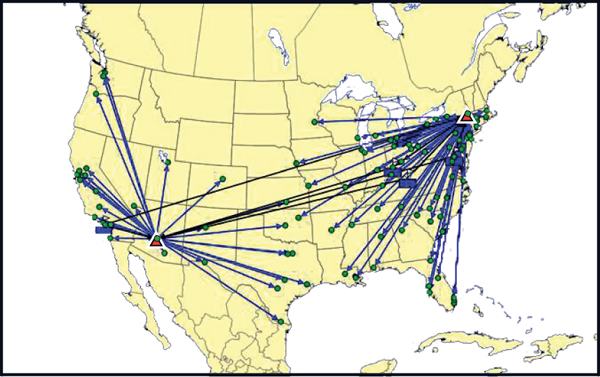
Figure 9.2. JADE’s Current Network Solution

JADE’s current transportation spend is $254 million per year, not including the additional cost to ship product from the plant in China to the port of Long Beach. Of this, $133 million is the cost to get product from the plants to the warehouses and $121 million is the cost to get product to the customers.

The new VP is convinced that they can reduce these numbers in the future. A quick look at the current state map shows that both of their warehouses serve very large territories for such a heavy class of products. In fact, a detailed analysis shows that only 21% of the demand lies within 200 miles of their current warehouse locations. Furthermore, only 32% of demand is within 400 miles.

Before we solve the JADE case study, let’s explore this type of problem in general.

Determining Warehouse Locations with Fixed Plants and Customers

To help us analyze JADE’s case, we will start with the simplest and most common three-echelon problem: locating warehouses given fixed locations of plants and customers. A model with a set of fixed customers is nothing new; all models in our previous examples had this basic assumption. Now we want to add a set of plants to the model where product is produced. Each plant may make different products or the same set of products. To start, we want to determine the best number and location of warehouses to minimize cost.

In this model, the plants ship to the warehouses and then the warehouses ship to the customers. We will assume that the plants cannot ship directly to the customers. This is very common in practice. Shipping direct to the customer requires a different set of systems and processes than shipping from a plant to a warehouse. For example, most plants are set up to produce large batches of a product. After products come off the production line, they are packed on to large pallets which are loaded into full trucks and shipped to a warehouse. When shipping to customers, a facility would need space to assemble the orders including the ability to put different products made by different plants on to a pallet or case for the customer. The facility would also need the ability to ship to its customers in various modes such as truckload, less-than-truckload, and parcel. Many plants do not have the space or capabilities for any of these requirements.

In addition, in many cases, the supply chain manager cannot consider changing the locations or capabilities of the plants. The plant locations are fixed and are not going to change. These may represent supplier locations that we cannot change, plants that required significant investment and are very difficult to move, or plants that require specialized skills and a trained labor force, or, quite simply, the company may not want to consider the relocation of the plants at this time.

The number and location of the warehouses is often an easier decision for many firms to make. And, plenty of savings opportunities are often discovered by relocating warehouses.

What makes this network design problem different from those in our previous chapters is that now the location of the existing plants or supply points will have an impact on the optimal location of the facilities as well. In the previous models, the facility locations were “pulled” to be close to the customers. That is, the model tended to locate facilities close to customers to reduce transportation costs. Now, we have two forces pulling on the location of the facility—the customer demand and the supply points. Simply stated, we want to minimize the cost of shipments both to and from the facility.

The relative strength of these two forces depends greatly on the problem being solved. In general, it comes down to the relative cost difference between the inbound and outbound costs. To highlight this, let’s review our previous discussion on transportation costs.

Let’s start by assuming that we have truckload (TL) shipments from our plant to the warehouse. That is, we easily fill trucks directly from the production line and ship these large quantities straight to a warehouse. This is a fairly common assumption. The warehouse then ships less-than-truckload (LTL) to customer points. That is, the customers order in smaller quantities that require this more-expensive transportation mode. Remember that on our cost-per-ton-mile estimates (the cost to drive one ton of product one mile), LTL transport is approximately three times as expensive as TL.

Let’s understand how this impacts the optimal location of a warehouse. Take a look at Figure 9.3. In Case #1, the plant ships via TL a short distance to the warehouse. The warehouse then ships the product to the customers via a fairly lengthy LTL shipment. In Case #2, we have the same set of customers, but the warehouse is much closer to the customers. Therefore, the plant has a relatively long shipment to the warehouse but, in turn, a short shipment to the customers.

Figure 9.3. Optimal Warehouse Location Visual

Which supply chain would you guess has the lower cost? We are assuming that everything else stays the same between the two cases. That is, we have exactly the same number and size of shipments. We have simply changed the location of the warehouse.

In this example, Case #2 will have the lower cost. In this instance, we are taking full advantage of the fact that TL is only one-third as expensive per ton-mile and are shipping the product to a warehouse as close to our customers as possible. So we are minimizing the total cost by maximizing the distance we ship on TL and minimizing the distance we ship via LTL.

If we extend this concept further and try to minimize the distance on LTL by adding a second warehouse (as shown in Case #3 in Figure 9.4), have we lowered the cost even further? To keep it simple, we will stick with our assumption that everything is the same between the two cases except the number and location of the warehouses. The customers still get the same sized shipments and the plant has enough volume that it can ship in full truckloads in both Case #2 and Case #3.

Figure 9.4. Optimal Warehouse Location Visual with Second Warehouse Option

Now, the answer is not as clear. For sure, Case #3 has lower transportation costs. But now we have a second warehouse. Presumably, this warehouse is not free. So now our answer to the question of which supply chain has the lower cost is “it depends.” It depends on the cost of adding that second warehouse. If the transportation savings offsets the warehouse cost, Case #3 has the lower cost; if not, Case #2 is better.

If we generalize this case, we can represent this graphically as a trade-off curve shown in Figure 9.5.

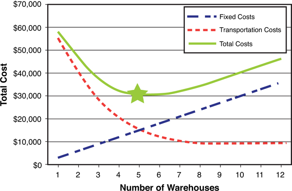
Figure 9.5. Number of Warehouses Versus Total Cost Trade-Off Curve

In this curve, you can see that the transportation costs decrease as additional warehouses are added. These additional warehouses also enable us to get closer to our customers and reduce transporation costs. However, as we add warehouses, the total fixed cost of the warehouses rises. This creates a total cost curve shaped like a bathtub. The best cost solution is at the bottom point of this curve.

Although this is a fairly common curve, each case will be different. In this case, being closer to the customers helped drive down the transportation cost but this is not always the case. For example,

• A plant may require a good deal of heavy raw materials for use in the production process. The resultant finished good sent out to customers, however, is relatively small and light in comparison. So the inbound cost may be expensive because of the weight and amount of inbound materials in relation to the cheaper outbound transportation of the lighter, smaller product.

• A retailer may ship full truckloads of a large assortment of its products to stores but source each product from a separate supplier requiring a lot of small shipments into its warehouse. As a side note, if these suppliers are widely dispersed geographically, they won’t have much influence on the location of the warehouses since the pull of the suppliers in the east will cancel out those on the west, for example. And, retailers also tend to put a lot more emphasis on the service levels they are able to offer to their stores. So, while being closer to suppliers might save them in transportation, they often choose to ignore this and prioritize the service level they offer to the stores instead.

The Problem and the Mathematical Formulation

For the multi-echelon problem in this chapter, we will add onto the previously developed models (especially the one in Chapter 7, “Introducing Facility Fixed and Variable Costs”), including capacities at the plant level. There are many possible extensions—here is one such extension. Note that, for simplicity, we renamed some of the constants because we now have explicit “warehouses and plants” instead of generic “facilities.”

A few notes on the model:

• Because we now have warehouses and plants, we added facility-specific prepends to certain terminology: whVar (the warehouse variable costs), pVar (the plant variable costs), transWC (the transportation cost from the warehouse to customer), transPW (the transportation cost from the plant to warehouse), whCap (the warehouse capacity), pCap (the plant capacity) and whFix (the warehouse fixed cost).

• The objective function here divides into three distinct sections. The first section computes the total cost of producing or acquiring our goods, and shipping them to the warehouse. The second section computes the total cost of handling our goods at the warehouses, and shipping them to the customers. The third section computes the total fixed cost of opening the warehouses. One isn’t obliged to organize the objective function in just this way. For example, we could have just as easily broken it out into five distinct sections, one each for production, plant-to-warehouse shipping, warehouse handling, warehouse-to-customer shipping, and warehouse fixed costs. So long as the correct total is computed, the objective function can be organized in whatever manner seems more readable and intuitive.

• The Z variable is new. This is the flow from the plants to the warehouses. This flow isn’t constrained to be binary—it can take on any nonnegative value. This is the first continuous variable we have used thus far. Note that if a particular type of MIP solver is used, and if demand and capacity values are all integral, then this value will naturally take on integral values.

• Equation (6) represents a family of constraints that is new to this book, but storied in the annals of network flow modeling. These constraints are called “conservation of flow” constraints, and they will appear in any reasonably sophisticated shipping model. “Conservation of flow” constraints transmit the obligation to ship and produce from the “sink” points (the customers) to the “source” points (the plants or suppliers). Without them, the goods would simply materialize at the warehouses, as they do in our previous one-tier models. Because the whole purpose of developing the more complex two-tier model is to allow the solver to include the plant production and shipping costs in the optimization decisions, these constraints are crucial. These particular constraints state that for each warehouse, the total amount of goods inbound from the plants must equal the total amount of goods outbound to the customers. The left hand side sums the inbound shipments over all the plant-to-warehouse lanes that terminate at this warehouse, and the right hand side sums the outbound shipments over all the warehouse-to-customer lanes that originate from this warehouse. By setting these two sums to be equal to each other, we insist that warehouses can neither consume nor produce goods, but merely act as conduits to enable more efficient shipping options.

JADE Case Study Continued...

Let’s get back to the new VP of supply chain and his need to quickly show supply chain savings for JADE. He had narrowed his ideas down to two main areas he felt had the potential for the largest savings for JADE. His first idea dealt with the optimization of the production network by determining the optimal product mix to produce at each plant location. The second was the optimization of warehouse locations and the customer service territory associated with each.

When considering which initiative to tackle first, he decided that changes to the manufacturing network would require more effort and take significantly more time to implement. He had found that each of their existing plants was very good within their current capabilities, and there was a level of risk associated with changing this product mix. He also presumed that there would be a lot of internal resistance to these types of changes. If he wanted to convince management of his ability to save JADE money, he concluded he should show results for the parts of the supply chain he could make changes to within a reasonable amount of time while causing the least amount of internal resistance possible. Therefore, his first objective would be to kick off a warehouse location study.

The analysis would start by reviewing differing numbers and locations of warehouses to service the JADE customers.

Transportation costs were by far the dominant cost in the warehouse network, so the VP immediately decided that the objective of his study would concentrate on minimizing that specific cost area only. All other warehouse costs were assumed to be negligible to the study. Based on what we previously learned about JADE’s network, we know that the trade-off that the VP’s study will be making is between the inbound cost and the slightly more expensive cost to transport product outbound to the customers.

The VP turned to a commercial network design application to facilitate his analysis. After loading all his data into the application, his first scenario was set up to select the best two locations, which he would then directly compare to the current two-location network being utilized by JADE.

Figure 9.6 shows the resultant optimal two-warehouse network. You can see that the model elects to move their original Phoenix warehouse servicing the West Coast only a slight distance to Las Vegas. The much more dramatic recommendation by this model, however, was to move the East Coast warehouse from New York to Columbus, Ohio. The VP was immediately able to understand this recommendation. Just by examining the map output, you can see that this new warehouse location is both closer to customer points and closer to the other plants.

Using these two new warehouse locations, the total transportation cost decreased to $196 million (from our original cost of $254 million). The cost to get product from plants to warehouses went from $133 million to $94 million, while the cost from warehouses to customers went from $121 million to $103 million.

Figure 9.6. JADE Optimal Two-Warehouse Network

This solution also shows a slight improvement in the customer service JADE will be able to offer. The percentage of demand within 400 miles increased from 32% to 37%. Not a dramatic improvement, but the VP realizes that using only two warehouses will always greatly limit service-level capability across the entire country. To test for even further transportation savings and improved service, he decided to run additional scenarios allowing more warehouse locations to be added to the network.

His analysis of the best three, four, and five locations resulted in the warehouse selections shown in Figure 9.7.

Figure 9.7. JADE Best Three-, Four-, and Five-Warehouse Solutions

As a result of these scenarios, the VP quickly prepared the table shown in Figure 9.8 comparing the costs within each.

Figure 9.8. Best Warehouses Scenario Cost Comparison

His first insight is in regard to the significant savings by just changing the location of warehouses. Simply moving the two warehouses to more optimal locations reduces transportation costs significantly. Adding more warehouses then only continues to reduce the cost. It is quite clear that JADE needs to change the structure of their supply chain.

However, before we jump directly to the VP’s final answer, let’s review some of the deep insight into JADE’s supply chain problem that this small set of data actually provides.

First, although we modeled only transportation costs, we gained some nice insight into the warehouse fixed cost as well. As we go from the best three warehouses to the best four, we see savings of $6 million. Therefore, we can conclude that if a new warehouse costs more than the $6 million, it would not make sense to open the fourth warehouse. Or, alternatively, if we cannot recoup the cost of moving into a fourth site with $6 million in annual savings, this move is not worth it. So even though the model did not capture these costs, we have enough information from the model to make decisions based on these factors.

Second, note that the rate of savings decreases with each warehouse added to the network. Simply moving to the optimal two locations, we save $60 million. By then adding a third warehouse, we see savings of an additional $12 million. Continuing on to add the fourth and fifth locations, we see that savings are only $6 million and $7 million. Based on this data, we can quickly conclude that the incremental value of additional warehouses decreases.

Third, the actual locations of the warehouses change within each solution. Sometimes, we get lucky and the optimal site locations build on each other from solution to solution. However, we cannot necessarily assume that implementing the best three locations now can be converted to the best four location solution later with the simple addition of one warehouse. If we want to eventually end up with four warehouses, we have two choices:

1. Pick the best three and add a best fourth warehouse later based on the original three locations as fixed within the model. This gets you a good solution for the best three, and if you never implement the fourth, you won’t have regrets.

2. Pick the best three out of the best four locations. If you are sure you will soon implement the fourth warehouse, this choice ensures that your fourth warehouse choice will be a good one.

Of course, as with all analysis, it is good to test both cases and see whether the cost difference is significant. The benefit in modeling is that these tests are free. If the cost differences are trivial, there is no reason for debate about the risk of each of the previous options.

Our fourth insight is that the savings of additional warehouses correlates directly with the savings in the warehouse-to-customer shipment costs. Because of the relative cost difference between plant-to-warehouse ($0.07 per ton-mile) and warehouse-to-customer ($0.12 per ton-mile) transport costs, it is always better to have more warehouses and locate them close to customers. Additional warehouses drive down the warehouse-to-customer costs, but you do pay for this with additional ton-miles going from the plant to the warehouse.

Fifth, we also see an increase in percentage of customers within 400 miles as the number of warehouses within the network increases. The model has no set parameters in regard to this data; however, the information is virtually free within our analysis. As determined previously, transportation costs decrease as we get closer to customers; therefore, improvement in service levels (proximity to demand) is directly correlated. This natural correlation among scenarios brings us to another good lesson, however: There may be an objective that is important to you (demand within 400 miles), but if this objective is not included in the optimization, there is no guarantee that the correlation will remain true across all scenarios.

Based on everything we learned previously, we should always remember to be careful about the assumptions we make. Assumptions are always made in these models. If the model did not include assumptions, it would likely be as complicated and costly as the real world and do us no good for the purpose of strategic analysis and efficient decision making. A key assumption in this model, for example, is the cost per ton-mile for our various shipments. Let’s test the logic of this assumption and see how it holds up.

The cost for warehouse-to-customer transit was developed by analyzing the current delivery costs to each customer. Presumably, each customer receives products from only a single warehouse, so this means that the order size and therefore shipment size will not change. In addition, as we add warehouses, logically this will lead to more short-distance hauls. Therefore, the minimum charge we have in the model helps protect us from assuming artificially low costs due to short-distance hauls. Based on these considerations, we can have confidence in these numbers.

The plant-to-warehouse assumptions may need more questioning, however. The validity of these rates depends on filling up the rail cars and trucks running on these lanes. If each plant is shipping to too many warehouses, however, it becomes more difficult to fill railcars and trucks. In this case, we can further test the ability to fill railcars and trucks by analyzing the annual flow of product from each plant to each warehouse. For instance, a total of 13 million pounds of inbound product from plant to warehouses translates into 250,000 pounds per week, which still should mean we can easily fill up our railcars and trucks with up to five total warehouse locations.

13,000,000 / 52 weeks = 250,000 lbs moving per week

250,000 lbs transferred to up to 5 warehouses = Average of 50,000 lbs to each warehouse

50,000 lbs > 45,000 lbs capacity of rail and truck transit modes

After reviewing the warehouse location scenarios and the amount of insight the VP of supply chain is equipped with, he is now in an enviable position. There are significant savings opportunities. He knows the major trade-offs, what information he gets free, and the limits of his current assumptions. Even under these circumstances, however, he still feels the need to run more scenarios to finalize his decision. You can assist him with these scenarios by completing the end-of-chapter questions.

Plant Locations Considering the Source of Raw Material

Similar to warehouse location studies, a network design study can help locate plants. In these cases we often want the location of suppliers or raw material to influence the location of the plant.

When transportation costs are important, you want to look at the same trade-off you looked at with warehouses: the difference between inbound and outbound transportation. That is, if it is expensive to ship product out of the plant relative to the cost to ship raw material into the plant, then the plant locations will likely be pulled closer to the customers.

One interesting difference, however, relates to our previous discussion around a plant receiving greater levels of inbound product compared to finished-good units being shipped out. In the warehouse examples already examined, we assumed that for each ton of product that came into a warehouse, the same ton was eventually shipped to the customer. For a plant, though, you may bring in two tons of raw material for every ton of finished good you ship out. In this case, you are still interested in the relative cost difference in inbound versus outbound transportation costs but now also with the extra influence of total tons being shipped.

Linking Locations Together for More Than Three Echelons

This three-echelon modeling logic also applies to networks containing more than three echelons. For example, let’s consider a business with the need for a hub-and-spoke type of warehouse structure.

Distributors often specialize in selling products sourced from thousands of small vendors. These firms add value to the market by consolidating shipments from all these vendors. The ability of the distributor to source and distribute this wide array of products as a single entity also simplifies the customer’s order process by allowing for the placement of just a single order for all needed items. The most expensive parts of a distributor’s supply chain are, most often, the collection of all the products from the numerous vendors and then making the final outbound delivery to the customer.

Because of this costly inbound as well as outbound transport, it often makes sense for distributors to locate multiple levels of warehouses. As shown in Figure 9.9, we see that the first set of warehouses collects products from the vendors while the second set is responsible for the final delivery to the customers. In the middle, the company can efficiently move product in full truckloads between warehouse sets.

Figure 9.9. Hub-and-Spoke Network Depiction

When locating the first set of warehouses, there are two common strategies. The first strategy locates either a single or small number of central warehouses. Locating just a few centrally works well when the vendors have enough volume to ship in full truckload to one or a few points. The second strategy locates numerous warehouses close to vendors and those vendors then ship short LTL shipments into the closest warehouse. This strategy works well when the vendors cannot fill a full truck even when shipping to just one location.

When locating the second set of regional distribution centers, common practice is to select numerous locations close to customers. As we have seen previously, the company’s ability to transport product in full truckloads into these warehouses allows for the concentration on better service and shorter outbound LTL shipment distances to customer points.

For some companies, however, two echelons of warehouses may still not be an optimal structure. Think about a major retailer that sells product online. Consumer locations become people’s houses, and orders may be as large as an appliance or as small as a single DVD or a package of socks. Based on what we have previously learned about transportation, these small shipments can be expensive to deliver to the home, even with the existence of regional distribution centers. For larger items (like appliances), companies will commonly use small trucks making multiple stops in a small geographic area (like a town or part of a metro area). These multistop routes require a local presence to facilitate their local delivery process, however. For the smaller items, these companies may use small-parcel delivery services. But even so, the objective would be to keep the product on ground and in full trucks as long as possible to control costs. So in both previous examples we see the need for the location of a third and final set of local warehouses. These locations are meant to receive product from regional warehouses and ease the high cost of small shipments deep into their markets.

Because it can be expensive to operate a chain of fully stocked local warehouses, many firms, in practice, treat these warehouses as cross-docks. It usually works something like this:

1. Orders come in throughout the day for deliveries needed the next day.

2. After some cutoff time, the regional warehouse starts picking orders for the local warehouses. These orders are loaded onto a full truck.

3. Overnight, the truck drives to the local warehouse.

4. First thing in the morning, the product is moved from the regional warehouse truck onto the delivery vehicles.

This approach has the benefit of moving the product as far as possible on a full truck.

When firms ship small-parcel and are charged per package, it is often beneficial to employ a strategy called “zone-skipping,” which is analogous to the previous example. The “zones” we are skipping are the zones set up by the small-parcel carriers (UPS, FedEx, DHL, and so on). The more zones we have to ship through, the more expensive the cost per package. Now, if we have enough volume, we can fill up our trucks with the packages for a local market and drive these trucks straight to the parcel carrier’s local sort facility. Instead of our delivery trucks, we are giving the product to the parcel carrier’s delivery trucks.

The previous hub-and-spoke networks had fixed supply points. What happens when companies need to determine optimal plant locations at the same time? In this case, we quickly find ourselves with more than three echelons to include in our analysis. When we locate our plants, we want to consider the location of the raw material sources as well as the location of the warehouses. And when we locate the warehouses, we want to consider the location of the plants and the location of the customers. So, in this model, we would be locating both the plants and the warehouses simultaneously. But as you are becoming a skilled modeler, you must always evaluate the complexity of the models you are proposing and the complexity of the output it may provide.

It is common to encounter a supply chain analyst having more difficulty in analyzing and interpreting the results than in setting up the model. When a model returns many different decisions at the same time, it can be difficult to explain what happened, spot potential problems, and determine the appropriate alternative scenarios. These types of difficulties can easily derail an entire project, and no CEO is going to make changes to the network if those changes cannot be fully explained and backed up by clear analysis.

One of our main objectives in this book is to break down supply chain network analysis into simple models you can use as building blocks to facilitate learning and allow you to efficiently analyze your complex problems. By using a series of simple models, you may be able to more effectively analyze your model without losing accuracy.

In the hub-and-spoke example, the problem naturally splits into two problems. The first is locating the central warehouse close to the suppliers. As previously discussed, thanks to the ability to ship relatively low-cost full truckloads from the central to regional warehouses, we can locate the central warehouses independent of customer locations. In parallel, the location of the regional warehouses does not depend on the central warehouses either. Instead, it depends solely on the location of the customers. By separating the models, we have two models that we can easily analyze and understand.

Even expert modelers know that the key to good modeling is in keeping it as simple as possible while still producing the level of detail required for explaining the results and eventually implementing the suggestions. By starting simple, you will also benefit from a full understanding of each modeling capability before moving on to include more complexity. If you ever find yourself getting confused, your best bet is to return to a single subset or the simplest portion of the analysis and work your way through from there. Chapter 12, “The Art of Modeling,” will further build on this concept as well.

Lessons Learned from Three-Echelon Supply Chain Modeling

When modeling three echelons at the same time, we were introduced to a new trade-off between the inbound and outbound costs. The inbound costs to a facility will tend to pull the location close to the source of products. The outbound costs from a facility will tend to pull the location close the customers. The relative difference between the inbound and outbound costs will determine which side has more pull (the sources or the customers).

Once we understand the concept of three echelon supply chains, we can naturally extend our models to include any number of echelons. We just need to watch out for the extra complexity that we add.

End-of-Chapter Questions

You can find the JADE model as well as detailed instructions for reviewing and running additional scenarios for the JADE Case Study within the JADE Case Study Exercise.zip file on the book Web site. Follow the directions within the JADE Intro Case.ppt file to open the model and review all input and output files to start. Then use this basis as well as additional scenario-building instructions to answer the following questions:

1. Based on the results seen previously in this chapter, as well as your running of these scenarios on your own through the model and PowerPoint referenced previously, review the new locations selected as the model solves for scenarios with two to five optimal warehouses and then explain:

a. How much impact did the change from Phoenix to Las Vegas have? Why?

b. What is the rate of change in the savings as each additional warehouse is added?

2. In the model, why would you expect the costs to continue to decrease as you add warehouses? In reality, would you expect this to hold up? Why or why not?

3. In the five-warehouse solution, even though the Columbus warehouse is very close to the plants, it still chooses to serve customers from additional warehouses. Why? In other words, why not save on inbound transportation and serve most customers from Columbus?

4. What if we wanted to implement five warehouses in the future, but wanted only four now. What is the cost of the best four, plus adding one more, versus the cost of picking the best four out of the best five? Which solution would you recommend?

5. Even though we don’t have the cost of opening a warehouse in the model, what information does the model give us in terms of what this cost needs to be for these solutions to be effective?

6. What are the optimal three warehouses and network total cost if all product comes from China (enter through the Port of Long Beach)?

7. What would have been the cost if they moved all production to China, but still chose our previous optimal three-warehouse solution (dual sourcing product)?

8. What is the value if all plants could make all four products? How much better of a solution could you derive?

9. Assume that the CEO is not sure whether all product will come from China but is sure that all plants will not make all products. What is your recommendation to the CEO for the location of the best three warehouses? Prepare three or four slides and be ready to present your result. You have to make a recommendation, but you are free to show other alternatives and discuss their merits. If there is missing data or information, feel free to use whatever assumptions you want, but make sure that those assumptions are as realistic as possible.