10. Adding Multiple Products and Multisite Production Sourcing

In the previous chapters, we have focused on various aspects of network design, including center of gravity models, service levels, and transportation cost modeling. All of these are key elements to understanding network modeling. However, we have yet to focus on differentiating between various types of products as they move through the supply chain. In this chapter, we will look at adding multiple products to the analysis and understanding its importance as it relates to network design.

Why Model Products?

Firms typically have thousands if not tens of thousands of products or SKUs that they manage and distribute through their supply chain. As we have seen in previous chapters, it is often common practice to use overall product weight to represent their movement within network models. We are in essence trying to estimate and represent the transportation costs associated with moving these products to meet customer demand. And as we have learned, transportation costs are heavily impacted by weight. Therefore, for modeling purposes, the appropriate costs will often be captured if we ensure that the total weight is accurately represented in the model. This also assumes that all products are rated uniformly using the same transportation rates. If that holds true, it is safe to assume that our results would be equivalent when modeling this weight moving in the form of 1 generic product or 100 defined products.

However, in this chapter we will learn that there are several cases where modeling a generic product may not be appropriate—in fact, when doing so, our model may yield incorrect results. These cases include the following:

• When our overall pool of products includes large variations in storage and logistics characteristics

• When some product types require specific customer service levels and therefore require specific transport modes

• When products come from different source locations

Let’s review each of these cases in further detail.

Variations in Logistics Characteristics

As we have discussed before, firms typically carry and distribute thousands, if not tens of thousands, of SKUs across the supply chain. It may be likely that these SKUs fall within different product-family designations, each with its own distinct characteristics, therefore requiring the modeling of separate products to accommodate the logistical differences as well.

Let’s take the example of a retailer. The SKUs carried by the retailer may include dry packaged goods (such as boxes of cereals, cans of soup), fresh produce items (apples, bananas, lettuce and so on), and frozen products (such as frozen dinners, frozen vegetables, and ice cream).

Each of these product families may be distributed in similar types of packaging (cartons), and they may even have roughly the same product density. However, the storage and transportation requirements are still very different for each group of items. The dry packaged goods can be transported in regular dry van trucks and stored at normal room temperature in the warehouses and stores. Fresh produce and refrigerated items, however, require specialized trailers with onboard refrigeration units that maintain the right temperature to prevent spoilage during transport. The transportation rates for reefer trailers (trailers with onboard refrigeration units) are typically 10% to 30% higher than those of standard dry vans. Bearing this in mind, we will need to ensure that we separate this volume of products moving on lanes so that they can be modeled with the correct transit cost using these higher transportation rates.

The same parameters also apply when it comes to storage requirements in our models. It is much more expensive to set up and run a warehouse with temperature-controlled chambers for refrigerated and frozen products. As a result, it is common for firms to use a large network of warehouses for dry packaged products, but storing refrigerated or frozen products in one or two warehouses only, given the higher capital requirements needed to support this capability.

The same rules are true for products that are considered hazardous materials or “hazmat.” These products have special storage requirements in the warehouse, as well as special handling constraints for transportation, thereby incurring higher costs. To address these constraints effectively, we again must ensure that we separate their activity within models by representing these as separate products.

Products with Differing Service-Level Requirements

When products are modeled at an aggregate level for each ship-to location, the analysis would essentially look at treating the shipment of all demand to customers in the same way. However, the shipment methods and patterns may actually be very different when analyzed in conjunction with demand by product families.

As you can see in the example in Figure 10.1, there is a significant difference in demand distribution between the two product families. This information can help in better analyzing and developing an optimal distribution strategy. For example, it is common for firms to develop different distribution strategies for distinctly different types of product families. SKUs that are considered critical parts may require expedited service such as same-day shipping or next-day delivery. The rest of the product portfolio may be delivered through normal shipping methods. In this case, it would be important to break out and model these products separately so that the appropriate service level constraints can be applied and the right network strategy can be developed.

Figure 10.1. Example Showing Differences in Demand Demographics Between Product Families

Leading companies tend to treat their supply chain as a collection of multiple supply chains for the various product families. The best overall modeling strategy is to develop the right network and distribution strategy for key product segments, while making sure that this does not create a suboptimal network at an aggregate level.

Product Sourcing

The source for the product is probably the most overlooked and important reason to include multiple product groups in a model. In the model, we want to make sure products come from the correct locations. Including product sourcing as part of our product groups, we ensure that this happens.

Including product sourcing information in our product groups allows us to specify which products come from which plant and which products are allowed to come from multiple plants (and we can specify which of the multiple plants). This ensures that our model correctly models the flow of product from the source to the final destination.

Adding Products to the Model—Mathematical Formulation

There are many ways to formulate a model with multiple product families. The simplest enhancement to this, however, would be to add product indexing to various components of the supply chain. This model is quite sophisticated so the following detailed analysis should give you further intuition.

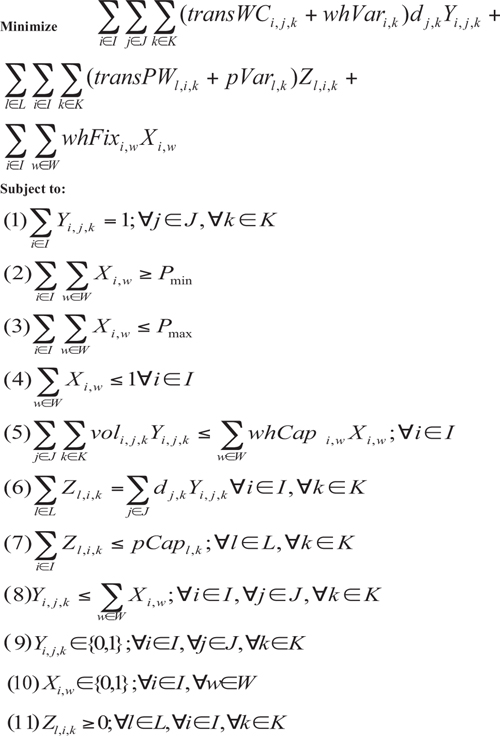
The objective function here consists of three components—the shipping from plant to warehouse, the shipping from warehouse to customer, and the warehouse fixed costs. (Note that in this model, we assume, for the sake of expediency, that plants cannot ship directly to customers. This useful extension, like many others, is not difficult to incorporate.)

The summation

captures the cost of shipping from warehouses to customers. We have many terms that are similar to those we have discussed previously, so it shouldn’t be very difficult to understand how this summation works. The set K represents our set of products (or, if product aggregation is used, our set of product families). We use the variable index k to represent a specific product (or product family). Thus, we use the term d_j,k to represent the demand for product k at customer j. We similarly capture the cost to process product k at warehouse i with the term whVar_i,k. The series of summations simply indicate that we are summing the warehouse-to-customer shipping and processing costs for every warehouse, customer, and product triplet.

The summation

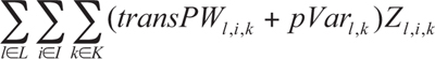
is similarly used to capture the cost of shipping from plants to warehouses. The term transPW_l,i,k is used to represent the cost of shipping one unit of product k from plant l to warehouse i. The term pVar_l,k is used to represent the cost of producing one unit of product k at plant l. The variable Z_l,i,k is used to represent the amount of goods of product k that are shipped from plant l to warehouse i. The summation indicates that we are performing this sum for every plant, warehouse, and product.

Note that Z is neither an integral nor a binary variable. That is to say, this variable is continuous. It is allowed to take on any value, such as 0.5, 100.3, or 1212.3. However, if we use one of the more common types of MIP solver engine, and all of our capacity and demand information is integral, then we know that any optimal solution will have an integral result for the variable. In practice, it is recommended that a user encourages integrality through this method, or, even better, simply rounds the results for shipping variables like this. Although there are more explicit methods of enforcing integrality on the per-product shipping variables, they almost always result in a significant increase in runtime.

The family of constraints

is very similar to the one we discussed previously. We are simply enforcing that a warehouse be selected as the service provider for each demand record. Note that we are prohibiting product splitting, but we are not enforcing single sourcing. That is to say, we will allow a customer to receive different goods from different warehouses, but we won’t allow a customer to receive the same product from more than one warehouse. It is possible to alter our model to enforce any of the logical combinations for these settings. That is, a customer might require single sourcing (and thus implicitly prohibit product splitting), allow multiple sources but not product splitting (as we do here), or allow product splitting (and thus not enforce single sourcing).

The constraint families (2) and (3) are not new. They simply require the model to select at least P_min warehouses to open, while ensuring that no more than P_max are chosen.

Constraint (4) has also been discussed before. It simply says that if a warehouse is opened, the solver must select one of the warehouse options from set W to build at this site.

Equation (5), while similar to a constraint family developed before, is worth closer examination.

In particular, we can draw attention to a few things. First and foremost, we note that the left-hand summation is over all the demand points (i.e., all the customer/product pairs). For a given warehouse, the left-hand side of this equation is the total volume of the goods being stored in inventory. The right hand side represents the size of the warehouse. The constraint family ensures that the warehouse will not hold more inventory than its size will allow.

Second, it is worth pointing out that the term, vol_i,j,k respresents the amount of space consumed by one unit of product k stored at warehouse j bound for customer i. It takes into account the following distinct quantities:

• The total demand of product k required by customer j. Although we have a distinct term d_j,k that captures this value precisely, we are blending this quantity into the value vol_i,j,k for simplicity’s sake.

• The physical dimensions of product k. For warehouse capacities, this quantity might be measured with something as simple as cubic volume or pallet positions, or it might be measured in a more sophisticated way that captures the efficiency of floor packing.

• The “inventory speed” of the warehouse. That is to say, a warehouse that frequently turns its inventory has a higher effective capacity than one whose goods linger for a long period. Because “inventory speed” (more formally known as inventory turnover ratio) varies from one product to the next, we need to incorporate this term into the vol term, instead of the whCap term.

This is just a cursory summary of how aggregate warehouse capacity is measured in a strategic network design model. We could write an entire chapter on this subject alone. For our purposes, it is sufficient to give you a sense of the complexity involved just in this one constraint family.

The constraint family

captures a well-known type of constraint called “conservation of flow.” Essentially, we are saying that the warehouse can neither create goods nor consume goods. Instead, goods enter the warehouse and leave the warehouse in equal quantities.

The left-hand side of the equation, , captures the total demand of product k inbound to warehouse i. The right-hand side, , captures the total outbound shipments of the same product. By forcing these two sums to be equal for every warehouse/product pair, we ensure that a warehouse is allowed to neither create goods nor consume them.

The constraint family

ensures that our plants are not used beyond their capacity. We are applying a capacity at the plant-product level. That is to say, we are ensuring that plant l cannot produce more than pCap_l,k units of product k. In industrial formulations, this constraint is often complemented by a plant-specific constraint that restricts some form of total production over all products.

Constraint families (8), (9), and (10) are very similar to those we developed previously. Constraint (8) has been modified slightly to ensure that a demand point cannot be assigned to an unopened warehouse (as opposed to the previous formulation, which ensured that a customer could not be assigned to an unopened warehouse).

Constraint family

(11)Z_l,i,k ≥ 0;lL, iI, kK

simply insists that the plant-to-warehouse shipping variables be nonnegative. Note that, unlike constraint families (9) and (10), we do not insist on true integrality here.

We now see the importance of adding products to a model, as well as how the addition of products essentially adds another entity with its own set of unique variables. This allows for modeling additional constraints such as restrictions on which products can flow through each warehouse, as well as setting the maximum number of warehouses that a given product family may be stored within.

To further our understanding of the inclusion of products in a network model and evaluate the implications of the solution, let’s go through a case study.

Case Study—Value Grocers, Grocery Retailer

Value Grocers is a mid-size grocery retailer headquartered in Chicago, Illinois. The retailer operates a network of 120 stores across the Midwest portion of the U.S. The retailer specializes primarily in an array of grocery items from frozen vegetables to juices and beverages. The company was founded in Chicago with one store operating out of a Lincoln Park neighborhood on the north side of Chicago. Based on the success of their first store, the founder decided to expand into other parts of the city. The business continued to grow aggressively over the next decade, and the Value Grocers’ store network expanded throughout the Midwest region, including store locations in Wisconsin, Minnesota, Iowa, Michigan, Ohio, Indiana, and Kentucky. The map in Figure 10.2 shows the current store network.

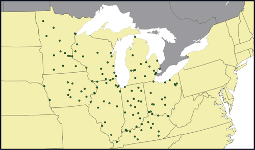
Figure 10.2. Value Grocers Store Locations

The company currently operates a single large warehouse in Chicago, which was set up originally when the company consisted of a small network of stores within the Chicago area. Despite geographic expansion across seven states over a decade, the company continues to serve all stores from this Chicago warehouse.

With the increase in fuel prices and overall transportation rates, the management team has become concerned about the growing logistics spend. With increased consumer focus on product freshness, the management team was also interested in increasing service levels so the stores could be replenished faster. Keeping these objectives in mind, the management team decided to initiate a network analysis to evaluate using additional warehouses to serve their stores.

For simplicity, we will use a representative set of products that are stocked and distributed by Value Grocers:

• Frozen products—for example, frozen beans, frozen corn

• Bottled juices—for example, pineapple juice, orange juice, apple juice

• Canned/bottled beverages—for example, soda and diet soda

• Packaged goods—for example, cereals, bread, nutrition bars

At first glance, it might be tempting to consider all of these items as one “grocery” product and focus on the total weight shipped from the Chicago warehouse to each Value Grocers store. However, these items have largely differing storage and logistics characteristics that require us to model several product groups as opposed to one flow of goods. We should first note that the frozen products and chilled juices require a temperature-controlled environment during storage and transportation. Therefore, as previously discussed, we will need to ensure that we reflect the higher transportation rates associated with the reefer (refrigerated) trailers that will be required to transport them.

Understanding the Impact of Product Dimensions on Transportation

In addition to the temperature requirement differences, let’s review the products’ dimensional characteristics as well. The table in Figure 10.3 shows the unit carton weight by product family. Looking at this information, we see that juice and beverage items are heavier, most likely due to their high water content, whereas cereal boxes and baked goods are relatively lighter. Why is this important to us? Let’s do a small side analysis to get a better understanding.

Figure 10.3. Weight (Lbs) per Carton for Key Product Families

Let’s first assume that all product groups are packaged in similar sized cartons—each with a volume of two cubic feet. If we were to fill up an entire truck with cartons of any one product family, how many cartons could be loaded based on their dimensions?

All trailers have a maximum capacity in terms of weight and cube (volume), and the true capacity is based on whichever limit is reached first. Let us assume that the maximum weight limit for the trailer (53’ trailer) in this example is 40,000 pounds, and the maximum capacity based on volume is 4,000 cubic feet.

The results of this initial analysis are shown in Figure 10.4. For fresh juices, we can load a maximum of 1,333 cartons based on weight and a maximum of 2,000 cartons based on cube. This means that we will hit our weight limit before we hit our volume limit and therefore can load a maximum of only 1,333 cartons within each trailer for distribution. We can also refer to this as “weighing out”—a common industry term for heavy products that are constrained in transport capacity by weight limits.

Figure 10.4. Product Characteristics Versus Truckload Capacity

On the other hand, cereal and baked-goods products will hit the max capacity based on volume (i.e., 2,000 cartons versus 3,333 cartons). These types of product are considered to be “cubing out” because they are lighter in density.

So how do these cube and weight differences impact our network model? As we know by now, transportation costs by lane is a key input into our network models. The weight and cube characteristics just reviewed will affect the amount of product that can be shipped for each iteration of truckload cost and therefore will also impact the transportation cost per unit calculated and used by the model. Figure 10.5 shows the calculation of transportation cost per unit for our data.

Figure 10.5. Transportation Cost per Unit by Product

For this example, if the truckload cost for a given lane was $1,500, the transportation cost per unit for canned beverages could be calculated as $1.35/carton ($1,500 / min [1111, 2000]), and cereals and baked goods would cost $0.75/carton. This leads us to easily conclude that it would cost almost 80% more per unit to ship a carton of canned beverages versus a carton of cereal products.

The previous analysis helps us, as modelers, in a couple of ways. First, it allows us to understand how to accurately calculate and represent transportation costs for these products. Second, this difference in unit transportation costs we discovered will directly impact several cost trade-offs in our analysis, and thereby impact where and how many warehouses these products are served from. We will revisit this topic in more detail later in this section.

To summarize, we can now firmly conclude that it is important to our model that we differentiate between several different product families in this analysis—not only due to the products’ varying temperature requirements but also because of their widely varying per-carton product weights. For simplicity, we will model four product families in this model—each product is actually an aggregated representation of hundreds of SKUs within the respective family. We will cover aggregation strategies in more detail in subsequent chapters.

Distribution Network Analysis Based on Outbound Flow

Now that we have defined our products, we can estimate demand by product and store and include this in our model. The map and chart in Figure 10.6 show a demand map with each store (represented as circles) sized by its relative product demand, and a bar graph showing total demand by product. The map highlights that Illinois, especially around metropolitan Chicago, still represents the high-demand areas—not surprising given the history of the company in this area. Stores in large cities such as Minneapolis, Detroit, and Cleveland also represent larger demand points compared to those in the non-urban areas. This is likely directly attributed to the relative differences in population density.

Figure 10.6. Map of Demand by Store and Demand by Product

Next, we will add a list of potential warehouses to evaluate as part of this network. The transportation in this model will consist of two types of carriers—one representing the use of regular dry-van trailers, and one representing temperature-controlled reefer trailers. Both carriers represent full-truckload transport with an associated cost-per-mile rate and minimum charge. Figure 10.7 shows the higher per-mile cost associated with the reefer trailers. Both modeled carriers’ transportation capacities will be set as a maximum of 40,000 pounds or 4,000 cubic feet and the model will apply the capacity limit that is first reached by product family.

Figure 10.7. Transportation Rates for Delivery to Stores

We will now begin running several scenarios to test where the best one, two, three, and four warehouses would be located. Our first objective, within the best one-warehouse scenario, is to understand whether there is a better location than the current warehouse located in Chicago. Obviously, setting up a new facility would require capital investment and fixed costs. Only if the transportation savings are significant would it would make sense to relocate the existing warehouse.

By reviewing the output of each of our four scenarios (shown in Figure 10.8), we can make a few quick observations. Chicago is selected as the best single-warehouse location—this validates that their current warehouse is indeed the optimal location from which to serve all stores in a one-warehouse solution. We also notice that the model progressively selects warehouse locations based on large pockets of demand. For instance, the best two-warehouse scenario selects Madison to serve metro Chicago, Minnesota, Wisconsin, and Iowa, and Ft. Wayne is selected to serve Indiana, Michigan, Ohio, and Kentucky. The three-warehouse solution then splits the region into three distinct demand pockets, and the four-warehouse solution essentially locates a facility in each of the key urban centers of demand.

Figure 10.8. Summary of Results with Best One-, Two-, Three-, and Four-Warehouse Locations

All these observations were strictly based on what we can infer from the geography of the locations picked. Let’s now take a closer look at the cost impact displayed in Figure 10.9.

Figure 10.9. Scenario Results Comparison

The cost-comparison table shows the biggest savings can be realized when increasing from a single optimal warehouse solution to an optimal two-warehouse solution. While subsequent scenarios continue to reduce costs as we increase the number of warehouses selected, we see that the incremental savings for each decreases. This reduction in marginal savings is driven by two factors. First, the overall average distance to customers will continue to reduce with each additional warehouse added to the network; however, the service level information shown in the figure clearly highlights that the proportion of the overall mileage saved reduces from left to right. Second, the carrier minimum charge starts to become a factor in how much savings may be realized with additional warehouse locations when the average distance to stores falls below a certain mileage band. This means that the cost of the shipment will not reduce even if an additional warehouse allows for product to be placed closer to the store than in the previous scenario.

Although we didn’t include the fixed cost of each incremental warehouse within the model (we learned about the inclusion of fixed and variable costs previously in Chapter 7, “Introducing Facility Fixed and Variable Costs”), the transportation savings with the addition of each warehouse may now be easily compared against the fixed cost of each additional warehouse outside of the model. In this case, the management team made a general estimate that the fixed cost for a new warehouse would be approximately $2 million. This means that the savings found in our optimal three-warehouse solution would still outweigh the cost of the additional two facilities ($5.16 million freight savings versus $4 million warehouse costs). Within the optimal four-warehouse network, however, the transportation savings of $6.44 million are almost equivalent to the additional fixed cost for three new warehouses ($6 million). Given that the savings in distance to customer are marginal with a four-warehouse versus a three-warehouse solution (only 23 miles closer on average), it makes sense to decide that the three-warehouse network solution is the best recommendation for Value Grocers at this point. Implementing this solution translates into the addition of new warehouse facilities in Minneapolis and Columbus.

Adding Storage Restrictions for Temperature-Controlled Products

As we begin to look at the three-warehouse solution more closely, we see that all three warehouses within the network are used to store and distribute all product families to their respective stores. From a warehousing perspective, this means that both new warehouses will need to be configured with temperature-controlled rooms, which requires a significant capital outlay they hadn’t fully incorporated into their average new-warehouse fixed cost estimated previously. The management team now wanted to understand the impact of storing temperature-controlled products in only one warehouse in order to minimize these additional capital requirements.

Because our modeled products are grouped by family and temperature requirements can be directly tied to the family (temperature-controlled products such as frozen vegetables and juices may be cleanly separated from our other regular, dry products), we are able to easily add this constraint in our model. The chart shown in Figure 10.10 compares the total throughput by product by warehouse for our previous optimal three-warehouse solution to the new scenario with temperature-controlled storage restrictions. This graphic clearly shows us that the Chicago warehouse is selected as the best location to store and distribute all temperature-controlled products.

Figure 10.10. Throughput Comparison by Warehouse for Temperature-Controlled Products

The cost comparison in Figure 10.11 shows that the solution with a single warehouse with temperature-controlled storage capabilities costs $2.42 million more than our original three-warehouse solution. This cost increase is expected because these products will be served from one warehouse instead of three, thereby increasing the average distance to stores. Obviously, this increase in transportation costs must then be compared with the savings in capital associated with equipping temperature-controlled rooms for the other two warehouse locations. If the cost to do so is more than $2.42 million, we know that this is our better solution.

Figure 10.11. Maps Comparing Results of Best-Three-Warehouse Solution with and without Storage Restrictions

Based on the detailed analysis we just reviewed, the Value Grocers management team now has the necessary information to make the best decision on the optimal distribution strategy for each of its product groupings in the context of their entire network.

Addition of Product Sourcing

In the analysis we have done so far in this chapter, we looked at only the outbound distribution from warehouses to store locations. From a product perspective, however, we have yet to analyze or include where the products were sourced from and how they were shipped into these warehouses to begin with. As we discovered in the preceding chapter, introducing three-echelon supply chains, this leg of any supply chain network can have an impact on your distribution strategy.

To effectively analyze product sourcing, we need to analyze and accurately model products so that the differences in sourcing are captured appropriately. Let us continue with our Value Grocers analysis and understand how this information is incorporated into our network design study.

To illustrate this point, let’s take one product category, Fresh Juices, and show how it has an impact on the solution. (In reality, each product category has an impact, and we would need to consider all of them together.) Let’s take apple juice and orange juice as two specific examples. A quick analysis of inbound for these products shows that the apple juice products are being sourced from a vendor in Michigan, and orange juice products are purchased from a different vendor in Florida. In the U.S., apples are largely grown in certain key states including Washington and Michigan, whereas Florida is known for its oranges. It makes complete sense that the juice vendors, in turn, typically locate their plants close to these associated produce fields.

Value Grocers currently pays for this inbound freight from these juice vendors to its existing Chicago warehouse, so this portion of their network is important to include in our analysis. As we have learned in the previous chapters, when we look at three-echelon supply chains, the trade-off between inbound versus outbound transportation costs becomes an additional factor in determining the location of warehouses. In this case, the inbound costs from vendors in Michigan and Florida into the warehouses will be traded off with the outbound costs from the warehouses to the stores.

Before we start analyzing the impact of inbound sourcing, we will need to update the products in the model to break out the Fresh Juice product into apple juice and orange juice. Figure 10.12 shows the updated demand chart with demand for apple and orange juices, along with their product characteristics in the model.

For the purposes of simplicity and ease of analysis in this study, we will assume that all other products have local sources near each warehouse and therefore their inbound costs will be insignificant within this scenario.

Figure 10.12. Updated Products for Model and Overall Demand by Product

The apple juice vendor is located in Grand Rapids, Michigan, and the orange juice supplier is located in Ocala, Florida. Both vendors currently ship product in full truckloads into the Chicago warehouse. For this analysis, we will assume that these inbound transportation rates ($/mile) are the same as applied for outbound truckload shipments in our previous models.

Also for the purposes of simplicity and ease of analysis, we will ignore the restrictions on the number of warehouses that may store temperature-controlled products. In other words, we will compare these results with our original optimal three-warehouse scenario.

The outbound solution maps in Figure 10.13 show that the inclusion of inbound transportation costs for juice products has dramatically changed the selection of warehouse locations in the optimal three-warehouse solution. We see that the Minneapolis warehouse, originally serving the upper Midwest, has now been replaced by a warehouse slightly farther south in Milwaukee that serves both the Chicago/Illinois area and the Upper Midwest. The warehouse location serving the Ohio region has now moved north to Toledo, serving both the Ohio and the Detroit areas, and the third warehouse has been chosen in Louisville, Kentucky.

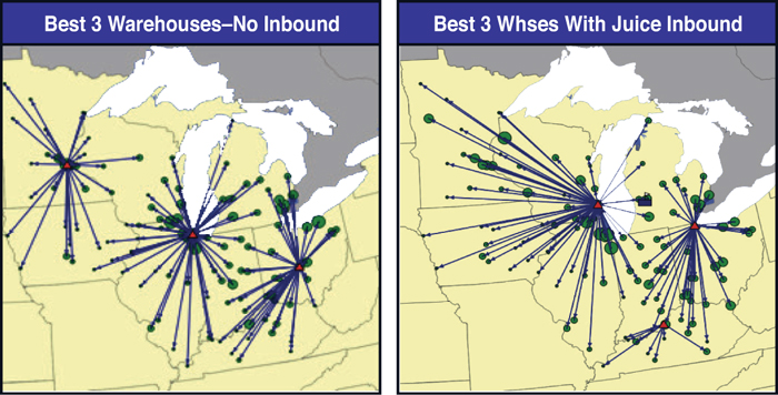
Figure 10.13. Map of Results for Best Three Warehouses—with and without Juice Inbound

What are the potential drivers of this drastic shift? Because we know that the only thing we changed from our previous solution was the inclusion of inbound transportation costs, we know this is the root cause of the changes in results. It is the result of inbound costs from Michigan and Florida that are pulling the warehouses both eastward and south based on the location of these vendors.

Before we look at cost comparisons between these scenarios, however, we need to run one more scenario that we can use as a fair comparison with this new scenario. Because the Chicago-Minneapolis-Columbus scenario did not include these inbound transportation costs, this scenario cannot be used as the basis of comparison with the new scenario. As a result, we will run another scenario with inbound juice transport and the original selection of Chicago, Minneapolis, and Columbus as the three-network warehouses, but allow the store assignments to be optimized. This scenario will then have the exact same cost components as our new scenario and can be used as an effective basis for comparison.

The table in Figure 10.14 shows that the Best Three Warehouses—Juice Inbound solution (Scenario C) yielded a total cost of $27.2 million. Even though we know that the models are not optimizing the same network objectives, we also see that the outbound cost associated with this solution (Scenario C) is significantly higher than the outbound cost for the solution without the consideration of inbound transport costs (Scenario A). We expect these results as the model is adjusted to now trade off inbound versus outbound costs, the result of which yields an understandably higher outbound cost.

Figure 10.14. Cost Comparison of Scenarios with and without Juice Inbound

The scenario results depicted in Figure 10.14 also show us that Scenario C results in a total cost only $0.6 million lower than the comparable original scenario utilizing the Minneapolis, Chicago, and Columbus warehouses but now also including inbound transportation costs (Scenario B). Inbound costs are lower in Scenario C than in Scenario B, revealing that Scenario C focused more on reducing inbound costs in relation to outbound costs in order to reduce the overall network transport costs. This is where the importance of analyzing both inbound and outbound costs simultaneously comes into play.

We continue our analysis of the impact inbound transportation on our solution, but will leave that to the interested reader to explore in more depth.

The Value Grocer’s case study has shown us the important of multiple product groups for more accurate costs (products fill up trucks differently), for different service requirements (frozen products), and for different sources (apple and orange juice).

Modeling Bills-of-Material (BOMs)

When a network design model includes raw material suppliers, the location of plants, and the decision of what product to make where, you will often need to include a bill-of-material (BOM). The BOM tells the model which raw material products are needed to make which finished good. That is, the model does not simply send the same product from the original source to the customer. The product changes form within the model as it moves from a raw material source to a plant and then on to warehouses or customers.

From a network modeling perspective, the BOMs are usually modeled as a combination of ingredients and processes depending on the scope and complexity of the manufacturing analysis. That is, you do not need to include every item listed in the actual BOM and need to think about how to model this effectively.

From an ingredients perspective, it is important to model only key ingredients that will impact the decisions on production sourcing based on costs and capacities. The BOM associated with more complex products may be quite lengthy and include many minor components (like nuts and bolts) that have no impact on results of the network design model. Therefore, our decision on what components or ingredients to include in a model should be based on the following:

• Contribution of Ingredient to Overall Product Cost

The focus should be on components that make up a large portion of the overall material or production cost of a product, and exclude components with low unit cost impact. For example, screws, nuts, and bolts may not be modeled, as they represent a very small portion of the product cost, and the change in production location will likely not have a notiticable impact on inbound costs for these components. Packaging materials may often fall into this category as well.

• Ingredient Sourcing Constraints and Its Impact on Finished-Goods Manufacturing

If there are specific components with sourcing constraints from a transportation or capacity perspective, such components should be included in your modeling. For example, key components that may be sourced only from a West Coast supplier may potentially impact the decision on producing the dependant finished-goods product in a West Coast plant versus East Coast plant. Similarly, any constraints on supply of ingredients such as availability based on seasonality or capacity constraints from specific vendors should also be considered. For a sugar manufacturer, for example, the sugar beets are harvested only during certain months of the year and must also be converted to raw sugar within a short time frame after harvest before they become unusable. Therefore, incorporating these timing constraints and relative importance of proximity to the source of the sugar beets is essential to any optimal solution in their network models.

Similarly, in terms of the production process, your focus should be on the modeling of only the key processes based on the following factors:

• Impact on Overall Throughput Capacity (i.e., Bottleneck Process)

Any given manufacturing process is typically made up of a series of production steps, each one performed on a specific type of production equipment. From a modeling perspective, the focus should be on the key processes that impact the overall manufacturing throughput for a given set of products through the plant—that is, the focus should be on the main bottleneck processes only, because this will directly impact how much product can be sourced from a plant overall. If we take the case of the manufacturing process for chewing gum, the bottleneck is usually within the sheeting process, in which the mixed gum (in paste-type form) is extruded and pressed through sheeting equipment to form thin sheets. This process is typically considered the bottleneck process, so the total volume of finished goods chewing that may be produced is largely dependent on how much sheeting capacity this equipment provides at each plant. As a result, this process should be modeled in the network model as part of the BOM.

• Impact on Key Capital Decisions

It is important to include processes that require expensive capital equipment and drive the decisions on what products to make in each plant. Note that this is focused on equipment that is directly tied to the production process for specific products, rather than equipment that is common to all products. For example, there may be certain tanks used to store byproduct liquids for disposal which are required for a production process but are not directly tied to any specific products. In other words, they are required for all products, and therefore will not influence which products are made at this location.

Bills-of-Material Example—Beer Manufacturing Process Modeling

To better understand the concept of bills-of-material, let’s look at the example of beer manufacturing. In this example, a beer manufacturer operates a network of four breweries across the country and is looking to optimize the production of finished-goods products (bottles, cans, kegs in various sizes and packaging types) across the four breweries. We will analyze the ingredients that make up the finished goods and the production process for the manufacturing of these beverages and packaging types, and convert this into a suitable schematic for modeling.

Many different ingredients are required in the production of beer. However, in general the key ingredients include water, barley, hops, and yeast (as shown in Figure 10.15). These are the key components from a production and product cost perspective but we need to carefully evaluate which ingredients are appropriate for modeling.

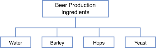
Figure 10.15. Overview of Key Production Ingredients of Beer

Let’s start with water. This is the most prevalent ingredient in beer in terms of weight and proportion. However, water is typically procured local to the brewery and usually doesn’t require shipping into the brewery from distant locations. So although this is a key ingredient, it does not add value as a component in a network model in this case because the water is always available to be sourced locally and at a relatively low cost to the overall process.

Barley and hops, however, are both typically shipped into the brewery from farms in ideal growing locations. Some BOMs may also utilize specific types of barley or hops in each specific type of beer. In this case we must model each of these ingredients in order to properly include the impact that their sourcing will have on inbound costs when determining where each finished good should be produced.

Lastly, yeast is probably the most critical ingredient in this process. The inclusion of a relatively small amount of yeast enables the production of alcohol from the sugar in the barley. Given the size and volume of yeast used in production, though, it is an ingredient that can be easily moved and shipped throughout any network at relatively low transportation cost. As a result, yeast is another ingredient that can be excluded from the network model, because it will not have a significant impact on our finished-goods production decisions.

Although we typically think about just products when modeling a BOM, we also need to consider the different steps required to make an item. Figure 10.16 shows the basic manufacturing steps for beer.

Figure 10.16. High-Level Overview of Beer Production Process

From a manufacturing perspective, this process can be broken into two main categories: brewing and packaging. Note that the brewing process is actually made up of several steps, including malting, milling, lautering, boiling, fermenting, conditioning, and filtering. However, from a modeling perspective, we want to focus on only the key processes that impact the overall throughput of beer production at each brewery. Each of the brewing process steps mentioned previously has its own production rate and throughput depending on the type of beer being produced, but they can collectively be grouped and modeled as an overall process in a network model.

After the beer is fermented, conditioned, and filtered, it is available for packaging into various types of packages—that is, bottles, cans, and kegs. The packaging process also requires additional product inputs in the form of packaging materials—that is, various sizes of empty glass bottles, aluminum cans, and kegs.

These packaging materials are sourced from specific vendors and shipped from each of their associated plant locations. More specifically, 12-ounce bottles may be sourced from one bottle manufacturing plant, while 16-ounce and 24-ounce bottles may come from a different plant. This inbound material sourcing will definitely impact the optimal production location for each of our finished-goods products, depending on where the packaging capability exists within the network.

In Figure 10.17, we show a sample schematic for modeling a BOM for several finished-good beer products in a network model. This BOM includes a combination of ingredients (hops, barley, and packaging materials) as well as production processes (brewing and packaging). This example could be expanded even further to include variations in different types of hops or barley that correspond to different types of beer as well.

Figure 10.17. Bills-of-Material for Model

When we have this information, we can build a network design model to incorporate it.

Whether it’s a network model incorporating the production of beer or one optimizing the production of computer chips, we can clearly see that the inclusion of production modeling requires us to not only differentiate our finished-goods products but also include raw material, component products, and the steps in the manufacturing processs within our analysis.

Lessons Learned from Adding Products

In this chapter, we learned the importance of modeling multiple products as well as the key drivers that make this a necessity for producing accurate results. These drivers include the following:

• Variations in logistics and storage characteristics that require us to be more detailed in our product definition in order to accurately capture the appropriate transportation and storage measures across the model.

• Products with differing service-level requirements require different modeled products in order to assign the appropriate transit time constraints as well as associate the appropriate transport mode and cost to each customer point.

• Variations in production sources and capacity constraints on the amount of product each source may provide require specific production definitions in order to track where each product may be sourced from and how much in an optimal network structure.

• Important raw materials or production steps. When modeling manufacturing operations, the source of the raw materials and steps in the manufacturing process may influence the results.

When additional product families are modeled, the solution can be driven by different products. For example, some product families may drive one set of facilities, and another set of products a different set of facilities. For example, if it is important to be close to the source of products, then the model may be pulled to locate facilities close to the source of Product A and also pulled to locate facilities close to the source of Product B. Adding products creates another internal trade-off that the optimization engine must balance.

The concept of modeling specific products within a network model is important for any company to understand. Not understanding this concept could leave a modeler with inaccurate results due to an inability to define all necessary costs and constraints specific to product groupings. Conversely, modelers may assume that product definition is always required when in actuality a lot of time could be saved while producing the same results for a model that doesn’t include any of our previously mentioned key drivers.

End-of-Chapter Questions

1. A popular online shoe retailer has been successfully servicing their customers across the United States with the most popular brands of shoes from tennis shoes to high heels for the past five years. The retailer sources these shoes from a wholesale shoe distributor and therefore receives all their shoe orders from the closest distributor stocking location. Due to the bulky packaging required to ensure no damage to the shoes in transit, the transportation cost is always volume dependent (or can be tied back to a per-carton cost).

The supply chain modeling team has previously modeled a generic volume of shoes flowing through their network to determine optimal warehouse locations. This year the company has decided to expand their retail footprint by beginning to offer the sale of designer formalwear such as suits and dresses as well. These products arrive in the supply chain on hangers and can’t be folded and shipped in cartons. The modeling team has determined that these products must be modeled as separate products within the network design.

Explain why this is a good decision in terms of transportation and warehousing cost differences.

2. Describe how you would model the associated products in each situation:

a. A German chemical company produces five different liquid chemical products (Liquid Products A through E for this example). These liquid products are often sold together in fifty-litre containers to regional manufacturing plants that in turn produce different blends of cleaning fluids then sold in the consumer market. Liquid Product B, however, is also a special chemical, essential to assisting with the emergency cleanup of oil spills around the world.

The modelers have decided to model two product groups in this case, one called regular and one called emergency. The regular product grouping consists of Products A through E, including the orders for Product B not for emergency purposes. The emergency product grouping consists of Product B, orders related to the emergency purposes only. Why is this decision appropriate?

b. A Canadian tire distributor sells thousands of different automobile tires to privately owned car-repair garages across the country. The distributor locations receive truckload deliveries of tires weekly from a single wholesale company operating one central distribution center in Canada. Each tire has a specific tread and thickness and thus requires a specific part number during ordering. The distributor has recently decided to expand its footprint to servicing markets in the U.S. and therefore is looking to complete a network design study to determine the best locations for two additional distribution centers within the northern U.S.

Why is this team able to model their network design problem with just one product group?

If this distributor decided to switch to sourcing its tires directly from the tire manufacturers instead of the wholesaler, they would then need to switch to include numerous product groupings in their model. Why is this? What would be the basis for these new product groupings?

3. Weighing Out Versus Cubing Out—Mini Case Study

Value Grocers has decided to expand its model to include product lines such as packaged deli meats and cheeses, crackers, potato chips, canned nuts, yogurt, and milk. You can find the detailed storage and logistics characteristics for each of our new product groups along with a sample model and detailed instructions for further analysis within the Value Grocers Expanded Product Line Exercise.zip file on the book Web site.

a. In the first model built, found in the file referenced above, we use only the weight of the products to determine transportation costs. What are the resultant transportation costs in the results of this model?

b. Let’s do further analysis to see how accurate these transportation costs might be. Using the Value Grocers Expanded Product Line Measurements.xls to start, complete your own calculations to determine which of these product groups will “weigh out” versus “cube out” (hit the max capacity based on weight or volume limits first) in real-life transportation costing. Remember that a single truckload of product can transport up to 40,000 pounds or 2,000 cartons of product.

i. Which products will weigh out?

ii. Which products will cube out?

ii. What is the resultant per-carton transportation cost for each product grouping based on this? What would it be if we didn’t differentiate between the products?

c. Back in our model, let’s adjust the model to include both the weight and the volume characteristics of each of our products, as well as apply both capacity constraints on the truckload carrier costs.

i. How does this impact our overall transportation costs within the model?

ii. Does this cause the model to select different optimal warehouse locations?

iii. Do certain product groupings tend to come from certain warehouse locations, or are product groupings fairly evenly distributed across the selected warehouses?

4. Product Sourcing—Mini Case Study

An Australian gold mine in Kalgoorlie (on the west coast of Australia) is used to supply gold to ten major jewelry-manufacturing customers on the east coast of Australia. The mined raw gold must be refined prior to delivery to these customers, however. This leaves the mining company with a need to determine the optimal location for this refinery. The mining company currently has two potential locations it is considering. The question is, should the refinery be located closer to the mine or closer to the customer base? To determine this, we must model the gold as both a raw material (raw gold) and a finished good (refined gold). A bill-of-material must also be modeled in order to determine the amount of raw gold required to produce one kilo of the resultant refined gold product used to service customer demand. The base model, as well as further detailed instructions for completing this study, can be found within Australia Gold Mining Product Sourcing Study.zip file on the book Web site.

a. In scenario 1 we define the BOM to mimic the fact that only 1.1 kilos of raw gold are required to produce 1 kilo of refined gold that can be used to satisfy customer demand. After reviewing the model setup, run the scenario and review results.

i. Which refinery is selected?

ii. What is the average distance traveled from mine to refinery? Refinery to customer?

b. Let’s create a second scenario but alter the BOM. Now the raw gold has a lesser quality and it requires 2 kilos of raw gold to produce 1 kilo of refined gold.

i. Does this change which refinery location is optimal?

ii. What is the new average distance traveled mine to refinery? Refinery to customer? Explain how the differing results in these two solutions make sense in terms of the amount of product moving on each type of lane (mine to refinery, refinery to customer) and the associated transportation cost changes for each scenario.

5. Bill-of-Material Modeling—Mini Case Study

Let’s consider the case of a chewing gum manufacturer that is interested in optimizing its manufacturing network and sourcing strategy. The products include sugar-based and sugar-free sticks of gum. Following is a quick description of the ingredients and the manufacturing process:

• Key ingredients include these:

• Gum base—Sourced from one of two plants worldwide

• Sweetener—Sugar or sugar-free substitute, sourced locally from regional suppliers at local prices

• Flavor additives—Very low weight, sourced from one flavoring plant in Seattle, Washington, for all gum manufacturing plants

• The manufacturing process starts with the use of mixing equipment to combine all ingredients into either sugar or sugar-free paste.

• The mixed product is then converted into thin sheets using an expensive piece of equipment called a sheeting machine. The sheeting machine also requires special parts to handle sugar versus sugar-free paste.

• In some plants, there are sheeting machines dedicated exclusively to each type of product (sugar, sugar-free).

• The sheeted products are then dried and cut into sticks.

• The dried sticks are then sent for final processing by packaging machines into any of several package types.

Let’s discuss the modeling of this BOM in terms of both the ingredients and the production processes.

a. The modeling team has decided to exclude the gum base ingredient from the BOM in their model. Why might this cause inaccurate results in their solution?

b. Based on what you know about the ingredients and production processes described previously, does each instance of the product (semi-finished or finished) need to be distinguished by their sugar or sugar-free nature? Discuss the specific effects on both modeling the production process and demand.

c. Is it essential to include the “mixing” step in the production process within the model? What might be the effect if it is excluded?

d. Is it essential to include the flavor additives in the model? What might be the effect if it is included or excluded?