
11. Multi-Objective Optimization
So far, we have discussed trying to improve just one component of the supply chain. That is to say, we have talked about minimizing the total distance that our goods have to travel, or the total supply chain cost over some length of time. We have framed strategic network design this way for three reasons:
1. Historically, strategic network design tools have always presented the user with a single goal. The majority of tools (although certainly not all of them) currently give you the power to minimize (or maximize) just one objective function at a time.
2. The mathematical tools that underpin strategic network design are oriented toward optimizing a single objective.
3. Optimization of a single goal is difficult enough to understand without the added confusion of considering multiple simultaneous objectives.
That said, the reality of strategic network design problems is that an analyst naturally gravitates toward more than one objective. For example, it is quite natural for a network design study to recommend the expenditure of a certain amount of upfront infrastructure costs in order to save money over a long time span. The analyst might conclude that significant savings can be realized by offshoring production to the Far East, and that two large West Coast seaports will be a key element of this plan. Although these warehouses will be expensive to build, they will more than pay for themselves over a ten-year time span.
Or will they? As this book is going to press, the price of electricity and natural gas (i.e., industrial energy) is much cheaper in the United States than it is almost anywhere else in the world, and Chinese wage inflation is eroding the cost savings of offshored labor. This combination is contributing to a trend of “reindustrialization” of the American Rust Belt. If this trend continues, a supply chain built just recently with an eye toward offshore production might completely lose its competitive advantage, and require reorienting toward more domestic production.
Of course, these sorts of trends are difficult to predict (if we could predict the price of energy, we could skip supply chain planning and make a fortune on the futures market). However, it is quite reasonable to consider limiting the amount of “upfront” fixed costs that our plans recommend. That way, if conditions change dramatically, our supply chain will not be locked into long-term lease payments on facilities that no longer make sense.
This naturally leads to a conundrum. We want to save money over a long planning horizon, because the most successful organizations invest in long-term success. However, we also want to reduce our fixed-cost capital commitments, because such obligations limit our ability to react to significant changes in the global economy. We have two reasonable goals that appear to be in irreconcilable conflict.
This sort of intellectual crisis isn’t limited to “upfront costs versus long-term savings.” It can also occur when one considers the trade-off between facility costs and customer-service level. When a customer is a long distance from the warehouse or plant that supplies it, the customer-service level will inevitably suffer. Sooner or later, the customer will experience a surge in demand that exhausts its in-store stock. If the supplier is nearby, an emergency restocking request can easily be accommodated. If the supplier is a long distance away, such a request might be impossible, or exorbitantly expensive, to fulfill. Thus, we might want to insist that every customer be sourced from a nearby facility.
However, such a requirement could radically increase the cost of our supply chain. In the most extreme case, we might end up building ten plants and 70 warehouses in order to service 120 customers. Such a large facility building and leasing expense could be quite significant, and completely dwarf the benefit from superior customer service.
Intuitively, this insight has a certain appeal. Customer service isn’t free. If we want 50% of our customer demand to be within 100 miles of a supplier, it might very well cost us more than a solution that places 40% of customer demand within 100 miles of a supplier. Although we can’t definitely answer which of these two solutions is “best,” it’s worthwhile to know the exact nature of the trade-off between these two choices. Even better would be to generate an array of worthwhile choices, each one representing a different trade-off between customer-service level and total cost.
Luckily for us, mathematical optimization has developed the tools to address the situation. The key is to recognize what it means for a solution to be worthwhile. More precisely, we will describe what would disqualify a solution from consideration, and then the set of worthwhile solutions will be those that cannot be disqualified.
Consider the “upfront cost versus total cost” conundrum described previously. Suppose an analyst generates three possible solutions to choose from (see Figure 11.1). The first solution costs $10 million upfront and $100 million overall; the second, $12 million upfront and $90 million overall; and the third, $11 million upfront and $100 million overall. The first solution is compelling because the upfront cost is so low, and the second is appealing because it represents a significant long-term savings. However, the third solution has no specialty to hang its hat on, as it has the same long-term cost as the first, but with a higher upfront penalty. Thus, we can safely disqualify the third solution from consideration, while the first two appear to be worthwhile.

Figure 11.1. Chart Showing Trade-off between Total Cost and Upfront Costs with Three Solution Points
More formally, mathematicians describe a multi-objective solution as Pareto optimal, if it is impossible to generate a “disqualifying” solution that improves on one objective without penalizing the other. In our example, if the first solution is Pareto optimal, there must not exist a solution with upfront cost less than or equal to $10 million and total cost strictly smaller than $100 million, and similarly there must not exist a solution with upfront cost strictly less than $10 million and total cost less than or equal to $100 million. Were such a solution to exist, it would be clearly superior to our first solution, as it would achieve at least as much long-term savings with a cheaper upfront cost, or it would generate a larger long-term savings with no larger initial outlay. A solution is thus Pareto optimal if no other clearly superior solution exists.
However, there might be many, many Pareto optimal solutions. For example, there might be four Pareto solutions, each with the following (upfront cost, total cost) values: ($10.5 million, $100 million), ($12 million, $90 million), ($15 million, $87 million), and ($19 million, $85 million).
These four solutions (see Figure 11.2) each represent different trade-offs between upfront cost and long-term savings, and thus, from a purely mathematical perspective, we can’t definitely say that any one is superior to the other. That said, it would not be surprising if the flesh-and-blood humans analyzing these four solutions decided that the second one is the pick of the litter. Its upfront cost of $12 million is quite close to the best upfront cost of $10 million, and its long-term cost of $90 million is quite close to the best long-term cost of $85 million.

Figure 11.2. Chart Showing Where the Four Pareto Optimal Solutions Sit on the Graph
Historically, strategic network design modelers have used “what-if” analysis to discover solutions that, though not provably Pareto optimal, are at least “close” to Pareto optimal solutions. That is to say, with the example previously given, a user might try to minimize total cost by optimizing three scenarios with three different upfront cost restrictions: “upfront cost <= $10 million,” “upfront cost <= $15 million,” and “upfront cost <= $20 million.” These results might play out as follows.
Scenario 1 is infeasible, because the upfront restriction was too tight. That is, there is no solution whose upfront cost is less than or equal to $10 million. Ideally, this infeasibility would be well diagnosed by a sensible error message, but in general, infeasibility diagnosis is quite hard.
Scenario 2 might generate our third Pareto solution with upfront = $15 million and total = $87 million.
Scenario 3 might generate a solution that is “close to” Pareto; that is, upfront cost = $20 million and total cost = $85 million.
Figure 11.3 shows how these three scenarios play out.
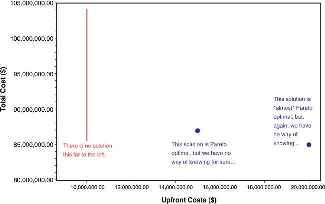
Figure 11.3. Chart Showing a Typical Result with “What-If” Analysis, Instead of Real Multi-Objective Analysis
We can thus easily see the imperfections of this time-honored what-if analysis strategy. The first problem is, simply, how do you determine the restrictions to apply to each objective? Clearly, our first scenario didn’t add much value, because its upfront cost restriction was unrealistically ambitious. Had we restricted upfront cost to $10.5 million, we would have discovered our first Pareto solution. However, when we’re starting from scratch, it might be no easier to realize that $10.5 million is a good what-if restriction than it is to determine next week’s lotto numbers.
The second problem with what-if analysis is that the solutions that it generates need not be Pareto. Consider the third scenario. Our solver engine minimized the total cost in this case while obeying the restriction that the upfront cost not exceed $20 million. In doing so, it discovered a solution that has total cost of $85 million and an upfront cost of $20 million. However, a clearly superior solution exists with the same total cost, and a smaller upfront penalty (Pareto solution number 3, which has total cost of $85 million and an upfront cost of $19 million). Why didn’t the solver generate this better solution instead? Because it was under no obligation to do so. Like any good computer program, it did what was asked of it—found the cheapest solution that doesn’t overrun $20 million in initial outlays. If we want our optimization tool to consider both goals at the same time, and thus uncover Pareto number 3 without any hints, we need a more sophisticated strategy than what-if analysis.
However, this third problem with what-if analysis is illustrated by what these three scenarios failed to discover. Specifically, what is arguably the best solution of all (upfront cost = $12 million, total cost = $90 million) was never generated. Although this solution will appear if we rerun Scenario 1 with an extra $2 million in the upfront budget, we have no particular reason to choose just this restriction. What-if analysis, by its very nature, is haphazard. Although it will give us some idea of what’s possible, it does a poor idea of telling us what’s not possible. Thus, a practitioner of what-if analysis is always left with some lingering doubt that the “Goldilocks”-perfect trade-off might appear if just one more scenario were optimized.
Luckily, better automated strategies exist. For some models, we might ask a particularly advanced tool to generate the full suite of Pareto optimal solutions; because such a suite might be large, our clever tool would likely graph the Pareto results, rather than present them as a flat list. That is to say, a graph might chart total cost on the y axis, chart upfront cost on the x axis, and plot our four Pareto solutions as dots on this graph (along with other dots for whatever other Pareto solutions exist). This is in fact what we have been doing with the graphs in this chapter—the strategy is so intuitive you probably understood it without any formal explanation.
However, this is, in general, an overly ambitious strategy. For some models, the number of Pareto solutions is so vast, with the differences between them so minor, that generating all of them might be pointlessly time-consuming. For other models, solving just one objective might be so time-consuming that it might be more realistic to simply remove large swaths of the upfront versus total cost graph from consideration. That is to say, it might be more worthwhile to graph what is and isn’t possible, and then let the user decide which sections need deeper consideration.
This is the strategy that commercial, off-the-shelf tools are following. A user will specify two objectives (i.e., total cost and upfront cost), and the tool will automatically draw two lines (or frontiers) on a bi-objective graph. This graph is seen in Figure 11.4. The upper line shows “what’s possible.” Although it might not be possible to create a solution that is “under and to the left” of this line, it’s certainly true that any solution that plots “above and to the right” can be improved upon. Similarly, the lower line shows “what’s impossible.” Although it might be possible to generate a solution that is inferior to a point on the lower line, it is impossible to generate any solution that plots “under and to the left” of the line as a whole. Thus, the “achievable frontier” (the upper line) and the “impossible frontier” (the lower line) can build intuition and help focus what-if analysis even in the early stages of optimization, when they are quite far apart.

Figure 11.4. Chart Showing Achievable Frontier (Upper Line) and Impossible Frontier (Lower Line)
As a multi-objective solve process progresses, it discovers more refined information about both what’s achievable and what’s impossible. This superior information is conveyed visually by redrawing the two frontiers. As new information comes in, the “achievable frontier” moves down and to the left, representing the discovery of solutions that have cheaper upfront costs or larger long-term savings. As new bounds are deduced, the “impossible frontier” moves up and to the right, representing the discovery that certain (upfront cost, total cost) pairs are unattainable.
For certain models, a user might realistically wait until the two lines completely converge (shown in Figure 11.5). Such a happy result would represent the discovery of the complete set of Pareto optimal solutions. These solutions would lie at the “L” corners, where the bottom of a vertical line segment meets the left end of a horizontal line segment.

Figure 11.5. Chart Showing That the Two Frontiers Have Almost Completely Converged
For most models, a true enumeration of the full set of Pareto solutions is unrealistic. However, such a perfect enumeration is hardly necessary. It’s quite easy to see that when the “daylight” between the two lines has been reduced to a mere glimmer, we have enough information to begin a comprehensive and orderly “what-if analysis” study. To return to our previous example, we don’t need the lower and upper lines to perfectly coincide to recognize that a solution very close to ($12 million, $90 million) is possible, and thus to launch a single optimization run with the upfront costs restricted to less than $12.05 million.
Lessons Learned with Multi-Objective Optimization
As we have previously seen, different objectives drive us to different solutions. In many cases, each of these objectives is important.
Multi-objective optimization is a technique that allows you to analyze two objectives at the same time to determine the appropriate trade-off.
End-of-Chapter Questions
1. If you run a multi-objective optimization and generate a Pareto optimal set of solutions, what work do you still have to do to determine the best solution for your supply chain?
2. If two large companies merge, why might you want to run a multi-objective optimization to trade off the total cost of company one versus the total cost to company two? That is, why might this be better than running with just the objective of minimizing the total cost of the combined supply chain?
3. Open the model and file Germany Store Delivery.zip on the book Web site. This file contains a multi-objective optimization for which the goal is to minimize the number of depots needed to serve stores in Germany such that as many customers are within 75km as possible. How many depots are needed to reach 50%, 60%, 70%, 80%, 90%, and 100% within 75km? If the management team thought they wanted 100% within 75km, how would this chart help you persuade them that this was not a good idea?
4. Let us revisit the case study from Chapter 10, “Adding Multiple Products and Multisite Production Sourcing,” for Value Grocers—the grocery retailer that operated a network of stores in the Midwest region. If you were to run a multi-objective optimization with this case study, what are the various objectives you would consider in this analysis?