
13. Data Aggregation in Network Design
In this chapter, we will focus our attention on one of the most interesting, yet challenging parts of network design—data aggregation (we’ll refer to it as just “aggregation”). Aggregation is putting the data of your supply chain into logical groups for the purposes of modeling. For example, instead of modeling every single item that moves through the supply chain, our model may contain only a small handful of product groups. When we aggregate, we typically aggregate the following:
• Products (from many different individual products to a small number of product families)
• Customers (from many different actual delivery locations to several hundred aggregate points representing all the customers in a geographic area with other similar traits)
• Plants, warehouses (that are a different building but on the same campus), and vendors (from hundreds of vendors to a small group of important vendors or vendors in the same geographic area)
• Time periods (modeling a year instead of every single day)
• Cost types (from many different line items to a single cost figure)
One of the reasons that aggregation is interesting is that it is both natural in how we think about problems and scary because we worry that we aren’t being accurate.
Throughout this book, we have used aggregation strategies without calling them out. Al’s example grouped all types of products into one weight based product group; the small-parcel example looked at shipments to about 200 customer points representing 10,000 or more actual shipment points; and so on. In each of these cases, we thought of the models as good representations of the supply chains. They seemed natural. Also, when we diagram a supply chain on a white board, we think of elements of our supply chain in groups. For example, we can draw flows for products that travel in full pallets and flows for products that travel in bulk containers. Again, all very natural.
However, when it comes to actually aggregating the data to make decisions, we lose our nerve, forget what is natural, and get scared thinking that if we don’t directly load all 10,000 products and 45,000 shipment points into the model, it won’t be accurate.
We need to get over our fear and learn the techniques of aggregation. Only firms that sell a very small number of products or ship to a small number of endpoints can avoid it. And even these firms may want to aggregate.
First, there are some technical reasons for why you want to aggregate:
• The optimization models we’ve covered in this book can be difficult to solve. If you simply loaded every product, every vendor, and every delivery point, you will likely find yourself with an optimization model that does not fit into the memory of the largest computer and has no chance of solving.
• If you are running a model for future decisions (and especially those more than several months or a year out), your forecasts at individual products or sites are not close to accurate.
On top of the fact that you technically can’t avoid aggregation (which, sadly, won’t be enough to convince some people), there are some very practical reasons you want to aggregate:
• Cost and time involved in obtaining, processing, validating, and analyzing data at a very detailed level is prohibitive.
• It can be impossible to understand the big-picture model and the influence and interaction between the key data elements if you are working at a detailed level.
• When the final decisions are made, the executives are going to go back to the natural way of thinking about the supply chain and think about the model in aggregate terms.
Because you cannot avoid aggregation, don’t fear it. When aggregation is performed well, models will closely represent the real world without sacrificing accuracy, but at the same time provide manageable and understandable outputs that lead to sound decisions.
Aggregation is also interesting because there is an art to it. The lessons we learned in Chapter 12, “The Art of Modeling,” also apply to aggregation. So you will need to use your creativity to solve problems. But there are also some best practices and science we can apply to make our aggregation decisions better. We will cover this later in the chapter.
Finally, this is interesting because there are many ways to approach aggregation and they may be different in each model or project. And the same business may use different aggregation strategies to answer different types of questions.
It is important to start thinking about aggregation early in the project—as early as the first discussions about the model. Following are some key questions to ask and consider to help drive the right strategies:
• What exactly are we looking to solve for, and what portions of the supply chain will we realistically be able to change? By answering this question, you can get a feel for which data elements are more or less important. If a data element is less important, it is a good candidate for aggressive aggregation. If you are answering questions about plant locations relative to warehouses that won’t change, it might make sense to roll all your customers to the warehouse that serves them.
• What data is available? If there are areas where you don’t have good data, you might as well aggregate.
• Are there detailed constraints to model? In general, the more detail you want to model in the constraints, the less aggressive you can be in aggregation. If you want to build constraints for just your top customers, you have to split your customers in a geographic area into at least two groups (one for the top and one for the others).
• How are the transportation rates applied? If we are looking at simple transportation structures, it may make no sense to add extra details. For example, if we are looking at minimizing the delivery cost of products from our warehouse to customers and all products travel in full pallets, then we might not need any detail on the products.
In the next few sections, we will introduce aggregation strategies for each of the elements of the model as well as discuss each of these strategies in more detail.
Aggregation of Customers
Customers are one of the most commonly aggregated elements in network design models. As a reminder, we are using the term “customer” to refer to ship-to locations, so if you ship product to a firm with ten locations, we are talking about the ten locations. A typical supply chain will include hundreds or thousands of customers to which products are distributed and where they finally get consumed. These sites may even change from year to year as the customer base shifts. Customer aggregation usually comes down to geographic proximity and types of customers.
It is pretty clear that customers that are physically close to each other should be grouped together. That is, if you have 25 customers in Denver, you might consider grouping these customers together. Then, if you have 3 distinct types of customers, you may split the Denver customer group into 3. You’ve gone from 25 points to 3 and still have the essence of your problem.
The most common strategy for grouping customers by geography is to use some form of the ZIP or postal code, or a metro area, or regional area.
For U.S.-based analyses, there are too many five-digit ZIP Codes, so it is most common to aggregate customers by three-digit ZIP Codes. (i.e., the first three digits of the standard five-digit ZIP Code). To pick the point to plot on the map, it is most common to use the largest single customer or five-digit ZIP Code. In general, there tends to be more three-digit ZIP Codes in largely populated areas and fewer in sparsely populated areas. The maps in Figure 13.1 show examples from Illinois and Montana.

Figure 13.1. Example Showing Aggregation at Five- and Three-Digit ZIP Level for Illinois and Montana
In the U.S., most transportation rate structures—especially small-parcel and LTL, are defined or estimated at the three-digit ZIP Code level. So, in one sense, you lose no accuracy by grouping by three-digit ZIP Codes.
In Europe, two-digit postal codes can be used like three-digit ZIP Codes in the U.S. Then, in all regions of the world, cities and regions can be good geographic zones. When doing worldwide studies, you may even aggregate all the customers in one country to a single point. Or if you have a model that is mostly focused on the U.S., you may aggregate your non-U.S. customers to the port of exit. The actual method chosen largely depends on the quality of data and how well it ties to the transportation rate structure. In some countries, aggregation to the district or county level may make sense if aggregation by city does not yield a significant reduction in the number of customers. Figure 13.2 shows the difference in aggregation at city versus district level for locations in India.
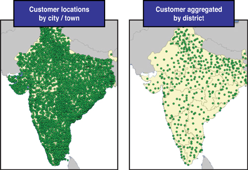
Figure 13.2. Example Showing Aggregation of Locations in India at City/Town and District Levels
For all models, it is very common to remove outlier and low-demand locations with insignificant demand that will always be difficult to service. For example, Alaska, Hawaii, and Puerto Rico in the U.S. are either modeled at the nearest continental U.S. port or excluded from the model. Or simply removing the low-volume demand points within your data may also save you time and effort.
In addition to geographic strategy, customers can be classified and aggregated using other key categories. You can think of this as stacking several points on top of the geographic aggregation. For example, if you aggregate by three-digit ZIP Code, you may have two points at each three-digit ZIP Code representing the two types of customers you want to model. Some examples of categories include these:
• Required service levels—For example, next-day customers and three-day customers. This provides the ability to identify and model different service levels and see the impact on the network strategy.
• Shipping methods—For example, LTL, TL, Rail. This allows the user to easily apply transportation rates and business rules by classifying customers that are served by LTL shipments versus TL shipments. See Figure 13.3 as an example.

Figure 13.3. Example Showing Breakdown of Volume by Customer by Mode
• Type of delivery location—For example, a store or an online customer. This provides the ability to track and apply specific business rules based on the type of end consumption point for the products.
You can be creative in coming up with customer categories. Just be sure you don’t create so many categories that you have more customers than in your original data set.
Also, don’t forget about the art of modeling and coming up with creative solutions. For example, there is nothing that says that when you decide to aggregate customers you have to aggregate all customers. If you have 20 to 30 customers that account for a large portion of your demand, you may simply model those customers as they are and aggregate all the others.
Validating the Customer Aggregation Strategy—National Example
We may need to validate the accuracy of our aggregation strategy before others in the organization will accept it. We’ll do two tests, one at a national level and one more detailed for a region. You may need to come up with other ways to validate your aggregation strategy.
This sample model has the following data elements:
• One product sourced from one plant.
• Our objective is to minimize transportation costs only.
• Consider two sets of potential warehouses:
1. 26 potential warehouses—major U.S. distribution points.
2. 60 potential warehouses—major U.S. cities/metropolitan statistical areas.
• For customer data we will use U.S. population data obtained from the U.S. Census Bureau Web site (http://factfinder2.census.gov/faces/nav/jsf/pages/index.xhtml). We will model this data at two levels of aggregation with this model:
1. Top 16,000 five-digit ZIP Codes with a population of at least 3,000 residents. We will exclude ZIP Codes in Alaska, Hawaii, and Puerto Rico for this example.
2. ZIP Codes aggregated to three-digit ZIP Code level. This yields a total of 876 three-digit ZIP Codes. For the model, we will pick the largest five-digit ZIP within each three-digit ZIP for geocoding.
• The total demand is the same in both cases.
For the first model, we will load data for 16,000 customers and 60 potential warehouses. For the aggregated model, we will load the model with the 876 three-digit ZIP Codes and the top 26 cities as potential warehouse locations.
The charts in Figure 13.4 give us a graphical view of the inputs for the two customer aggregation strategies. We can see the significant difference in density of customers between the two models. However, the real question is whether this increased level of detail offers any significant benefits in terms of the quality of outputs and associated decision making.

Figure 13.4. Comparison of Input Data—16,000 Versus 800 Customers
For purposes of simplicity, we are using a truckload rate of $2/mile and 40,000 units per load.
To test the models, we will run a scenario on each model to pick the best five warehouse locations from the given list of potential sites. The results of the two models are shown in Figure 13.5.

Figure 13.5. Comparison of Output Results
The charts themselves give insight into how the models compare. Both models picked the same five warehouses: Newark, New Jersey; Atlanta, Georgia; Dallas, Texas; Chicago, Illinois; and Los Angeles, California. This shows that with the right aggregation strategy, we can come up with the same answer as one without aggregation. The model with three-digit ZIP Codes is much easier to run and analyze compared to the unaggregated model.
Now when we look at the actual costs, we see that the aggregated model varies by only 0.363% from the model without aggregation. As noted in the previous example, it is likely that the forecasted demand has more error than the difference in these solutions.
By using three-digit ZIP Code level aggregation, our customer file went from 16,000 to 800 without loss of accuracy. This model was further simplified by reducing the number of potential warehouses, without any difference in the final solution recommendation.
Validating Customer Aggregation—Regional Example
In the previous example, we analyzed and validated the impact of customer aggregation on a broad, national level. In this example, we will focus on a specific market (Chicago) and see what kind of impact aggregation may have. This gives you a deeper look at the impact of aggregation.
The map in Figure 13.6 shows a set of 30 ship-to locations in the Chicago area, at the five-digit ZIP Code level. Each customer location receives between 5 and 20 full truckload shipments a week.

Figure 13.6. Customer Locations in Chicago Area, and Weekly Demand in Number of Truckloads
For this validation exercise, we will estimate the transportation costs to serve this weekly demand from a set of warehouse locations in Indianapolis, Indiana; New York, New York; Atlanta, Georgia; and Chicago, Illinois (see Figure 13.7). We will estimate the costs if these customers were to be served from each of these warehouses as potential options.

Figure 13.7. Map Showing Warehouse Locations and Customer Locations in Chicago Area
We will then aggregate these customer locations at the three-digit ZIP Code level, and recalculate the transportation costs from the same warehouse locations for the same total weekly demand. We can then compare the transportation costs for the two scenarios to understand the impact of this aggregation strategy.
Before we begin, let us look at how the transportation costs will be calculated. Because these customers are served by full truckloads, we will use a cost-per-mile rate applied against the distance to estimate the costs. For this example, we will use a cost of $2/mile as the rate for the truckload shipments. As noted in previous chapters, truckload carriers also apply a minimum charge for shipments that fall within a very short distance. For this case, we will use a minimum charge of $400 per TL shipment. This means that we will use the larger of the distance-rated cost versus the minimum charge. Because the warehouse in Chicago is one of the options, we can note that the minimum charge will apply because the distances fall within 200 miles.
The table in Figure 13.8 shows the transportation cost estimates by customer location (five-digit ZIP Code). We can see that the costs from Chicago to all customer locations are based on the minimum charge because the distances are less than 200 miles. For example, the cost for customer ID 1 (60016) is $400 * 10 truckloads, or $4,000. We also see that there are a few ZIP Codes that are less than 200 miles from Indianapolis and hence the minimum charge is being applied.

Figure 13.8. Transportation Cost Estimates for Customers at Five-Digit ZIP Code Level
Now, we will aggregate the customer locations to the 3-digit ZIP Code level for this exercise. The chart in Figure 13.9 shows the demand calculation with aggregating from 5-digit ZIP to 3-digit ZIP level. The total number of truckloads is maintained at 305 loads. We will use the largest 5-digit ZIP within each 3-digit ZIP for geo-coding in the model. So, the number of customer points in the model has decreased from 30 to 8.

Figure 13.9. Aggregation from Five-Digit to Three-Digit ZIP Code Level
We will use the same rate structure for this model including the minimum charge. The results of the analysis at the three-digit ZIP level are shown in Figure 13.10.
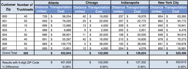
Figure 13.10. Transportation Cost Estimates for Customers at Three-Digit ZIP Code Level
The results show that the costs from each warehouse for the three-digit model are very close to that of the five-digit ZIP model. The differences are in the range of –0.29% to +0.40%, which is certainly smaller than the error in the demand forecasts or in likely transportation rate changes because of changing oil prices.
We also notice that there is no difference in costs from the Chicago warehouse as the minimum charge applies again for all locations. The differences in distances due to aggregation are eliminated due to the minimum charge. This is a key point to take note when aggregating at a regional level. Even though the five-digit ZIP level model shows a greater level of detail in actual locations, this does not offer any additional advantages in terms of costs.
To summarize, this validation exercise helped us understand how the right aggregation strategy can still provide valid and accurate results even at the regional or subregional level.
Aggregation of Products
Product aggregation tends to be more challenging than customer aggregation. With customer aggregation, it is hard to go too wrong grouping customers by proximity. With product aggregation, most firms already have products grouped into marketing families. Unfortunately, there is nothing about a marketing family that naturally makes it a good candidate for an aggregate product group for a supply chain model. For example, a retailer may have a marketing family for Women’s and Men’s Apparel. From a logistics viewpoint, it might be more natural to have the socks be in one product family because they may come from the same vendor, have the same relative size, and require the same shipping and handling methods. On the other hand, the hanging clothes may naturally fit together because they are shipped and handled together.
So products sharing logistics characteristics make for good product families in a network design model. The marketing families are often irrelevant.
This means that you, the supply chain team, may need to create new product families and have the people in the organization agree to their validity.
Before we go too deep into product aggregation, there are two key questions you should ask at the start of every project. These questions will save you a lot of time in product aggregation and may help you avoid complicated product aggregation exercises.
The first key question is this: Can you create one aggregate product representing everything?
If you think about this from a marketing point of view, you will never answer “yes” to this question. However, from a logistics point of view, if you care only about pounds, kilos, pallets, cartons, or boxes moving through the supply chain, you should use it. In the examples in this book, we showed legitimate models that relied just on total weight or total packages sent through the supply chain, with no details on the underlying products. In practice, many good models are built with one product family.
After thinking long and hard about the first question, the second critical question is this: If we can’t create one aggregate product family, will two do?
Of course, this question is really many questions, because you may want to ask about three, four, and so on. You can see that the preceding questions suggest a way of thinking about aggregation that will help you. We have found, in practice, that it can be easier to start your product aggregation with one aggregate product (say pounds) and then grudgingly add more products as needed. This is opposed to starting with all 10,000 individual products and trying to whittle it down. In the latter case, it is always harder to get to a manageable number of product families.
As you start to add more product groups, or your hand is forced, and you must start with all products and whittle it down, you need to know what characteristics to consider. What is important is that you consider the logistics characteristics of the products. The following sections provide some guidelines for how to group products.
Consider the Source of the Products
The source of the products is often the most overlooked category and can cause serious flaws in your model if you do not properly account for it. When including the source of your products, you are grouping products by where they came from. This helps ensure the correct flow from the plants to the final customers.
As an example, if you are building a model for the supply chain of apples, you could start by grouping all types and sizes of apples into one product called “apples.” However, if your red apples come from Michigan and yellow apples from Washington, you need to include this in the aggregation strategy. Customers will demand both red and yellow apples. If you group products into just “apples,” the customers close to Michigan will get all their apples from the Michigan orchards and the ones on the West Coast will get all their apples from Washington. There would be nothing in the model to force customers to get apples from both Michigan and Washington. To make this happen, you need to create a product grouping that includes the source. For example, the table in Figure 13.11 shows some of the types of apples in this example.
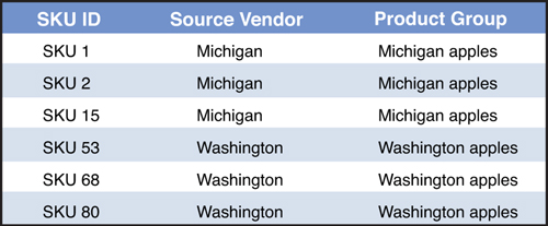
Figure 13.11. Example of Apple SKUs Categorized by Source Vendor Location
The correct way to model this would be to aggregate the three SKUs from Michigan as “Red Apples—Michigan sourced,” and the remaining three SKUs as “Green Apples—Washington sourced,” and allow only Michigan apples to come out of Michigan and the same for Washington. This will now correctly reflect the flow of products through the supply chain.
In more complex situations, a general way to think about categorizing products by sources is to think of sourcing groups. A sourcing group consists of all the SKUs or products that are made from the same set of plants. This structure allows you to capture the fact that products can be made in multiple locations. As an example, the following table shows how you might go about this task.
The table in Figure 13.12 shows that SKU 1 and SKU 8 are sourced from Plant 1, and therefore placed in Group 1. SKU 7 and SKU 12 are both sourced from Plants 1 and 2, and therefore placed in Group 1-2.

Figure 13.12. Categorization of SKUs into Source Groups
Consider Removing Products with Low Volumes
Part of the art of modeling is to separate the significant from the trivial. And, often, when a firm makes or sells thousands of products or SKUs, they will have many very low-volume products. The chart in Figure 13.13 shows a typical example of the number of products sorted from highest demand to lowest and showing the cumulative percentage of demand.

Figure 13.13. Product Demand Pareto Chart
When we analyze this, we immediately find what most firms find with their data: 90% of the demand flowing through the network is made of less than half of the total 500 products. Taking that further, we see that 99% of the demand is made up of only 100 more products, for a total of 300 products. So, 300 of the 500 products make up 99% of the demand, and we can easily remove the remaining 200 products from our analysis.
Consider the Size of the Products
The size of the products can impact transportation costs and warehousing costs. So products of similar size could be grouped together.
A perfectly valid and simple way to do this is to group products by small, medium, and large. As an example, in reality, this translates into products shipped in boxes, those on pallets, and bulk items.
A more sophisticated way is to cluster the products by their weight and cube (or cubic volume). This will help accurately model transportation costs while reducing the complexity of the model. The graph in Figure 13.14 shows an example of clustering.

Figure 13.14. Plot of Products and Their Respective Unit Weight
The graph shows a plot of the products based on their unit weight (lbs per case) and volume (pallets per case). The rectangles shown on the graph illustrate how to cluster SKUs based on similar weight and cube characteristics. There are sophisticated ways you can do this type of cluster analysis that are beyond the scope of this book. However, keep in mind that you want to try to keep your aggregation strategy as simple as possible.
Consider Different Packaging Requirements
It is also common to aggregate products based on their packaging requirements that may help easily model manufacturing and transportation costs. For example, the products for a beer manufacturer can be classified into bottles, cans, and kegs (see Figure 13.15). We can further classify bottles into 6-pack, 12-pack, and 24-pack, allowing the user to model specific constraints and rules for each package type.

Figure 13.15. Example of Beverage SKUs with Package Attribute
Consider Production Requirements
The same criteria can be applied to production requirements in order to simplify sourcing and production constraints and rules. For example, products that require special coating can be classified and tagged, allowing these products to be easily assigned to the specific production lines in the model.
Consider Products That Share Components or Raw Materials
Products that share the same components or raw materials can be aggregated together in order to simplify the modeling of bills-of-material and associated business rules for these products. A model for a chewing gum manufacturer would classify products as sugar and sugar-free based on products that use sugar or sugar substitute, allowing the modeling of sourcing rules.
Consider Products That Share Transportation Requirements
Products that require special transportation modes or requirements can be aggregated together to allow modeling of transportation rules. For example, products that ship in liquid form would be separate from the same product that may be put in a barrel first.
Consider Per-Unit Production Costs
In some supply chains, there may be several products within the same product family or group or across product groups that have significant variation in the unit production costs. This may be attributed to variations in some component or raw material, or the differences in the production process itself. Depending on how these other portions (raw material and BOM, production lines) are modeled, it may be easier to group the SKUs based on the unit production costs to simplify the modeling.
Consider Predefined Product Families
In some cases, if the company has experience with network modeling, the existing product families may work. Of course, if the firm has experience with network modeling, they likely will have gone through the steps listed previously.
For example, a retailer may classify its SKUs into frozen goods, dry goods, fresh produce, liquid beverages, and so forth. Or a beverage producer may group products as shown in the table in Figure 13.16.
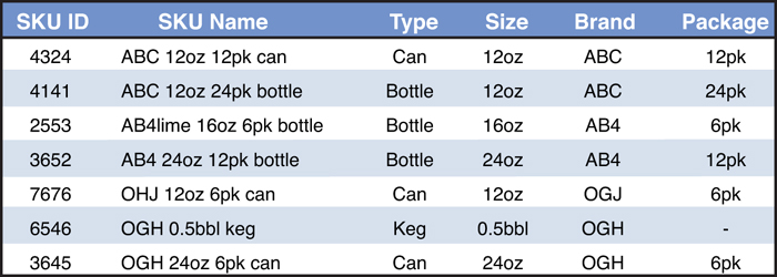
Figure 13.16. Example of Beverage Products with Key Attributes Useful in Aggregation
If this information is readily available, you should use it.
Testing the Product Aggregation Strategy
As a next step, we will look at testing an aggregation strategy in a model with some sample data. For this test exercise, we will build a sample model with the following elements:
• 25 potential warehouses
• Distance-based service constraints
• Inventory holding costs
• Fixed warehouse costs
• Product aggregation—we will test the model with the following options:
• 46 original SKUs
• 4 aggregated products—aggregated products were created using weighted averages and clustering (similar to the methodology used in a previous example)
The model was run with 46 products, and then with 4 aggregated products. The results of the two scenarios are shown in Figure 13.17. The analysis shows that the aggregated model was 0.0003% higher than the one without aggregation. The difference is that one model picked Seattle, Washington to cover the northern part of the West Coast and the second model picked a location in Northern California.

Figure 13.17. Results Comparison for 46 Original Products Versus 4 Aggregated Products
So the critical question is, Does the Seattle solution really differ from the Northern California solution? To understand this question, we will run two scenarios with each model: one scenario forcing Seattle and another scenario forcing Northern California. The results are shown in Figure 13.18.

Figure 13.18. Comparison of Results with Seattle and Northern California
If we look at the results for the model without aggregation, we see that there is a difference of 0.1% between the Seattle and the Northern California solutions. This difference is extremely small considering the margin of error and level of accuracy of the underlying data within the model. It is likely that the forecasted demand data has more error than the difference shown here. This helps us conclude that the Northern California solution is equivalent to the Seattle solution based on the cost factors analyzed in the model. This means that the solution requires further analysis evaluating other factors such as labor availability and logistics infrastructure.
This also shows that the aggregated model is still accurate given the margin of accuracy for normal models. The key take-away from this exercise is that with the right aggregation strategy, we can get the same level of accuracy in decision making as one would achieve with modeling without aggregation.
Aggregation of Sites
In most models, you have a limited number of plants and warehouses. So you usually keep these as individual sites and do not need to aggregate. The one minor exception is when you may have two to three plants or two to three warehouses that are all on the same campus or within the same city. In this case, as long as the facilities do similar things, you may group them together.
This is not always the case for vendors. Many firms have hundreds and maybe thousands of vendors.
If we need to include vendors in our model, we treat this a lot like we did with customers. We group vendors by geographic proximity and maybe by type. The example in Figure 13.19 shows vendors grouped by three-digit ZIP Code in Georgia, but we can often build good models by grouping vendors by a larger geographic area like a U.S. state, country, or even a port of entry. As another example, in a U.S.-focused model you may aggregate all your Asian vendors to a single point in Long Beach, California.

Figure 13.19. Example Showing Aggregation of Vendors in Atlanta Area
Aggregation of Time Periods
When aggregating time periods, we are simply determining the time buckets we will use for our model.
The industry standard for time-period buckets in network design models is a year. Within a year, you capture the full range of demand across seasons, and it is natural to think of reporting your costs and savings in terms of annual numbers. And the nature of most decisions about when to open or close a facility does not need more granularity than an annual bucket.
With this structure, nothing prevents you from running what-if scenarios with different demand patterns. That is, you can run a model with the expected demands five and ten years out. Even more so than with products, we want to make sure we are careful when we model more than a single annual time period.
There are two basic problems we solve when we include multiple time periods in the same model. The first problem we can address is to determine what year to open and close facilities. To capture this, we could model multiple annual buckets in the same model and have the model pick which year we open or close facilities. Note that this makes the model much more complicated. One way to avoid this complication is to simply run different what-ifs with future demand scenarios. You may think you are losing accuracy, but in reality, predicting demand several years out is very difficult anyway, so you may be just introducing false precision by including multiple years in the same model.
The second problem we can address is to determine how to handle seasonality. In this case, we may build models that have 4 quarterly buckets to make different decisions in different parts of the year. Or if the prebuilding of inventory is important, we may model in 12 monthly buckets.
For example, if we look at a consumer products company that experiences a high spike in demand in the summer, we may want to make decisions about when to start building the inventory and where to store it. The graph in Figure 13.20 shows the spike in demand and the need for extra storage capacity.

Figure 13.20. On-Hand Inventory Versus Warehouse Capacity
These are some general rules for thinking about time periods. As with all modeling, you can get creative to solve your specific problem. For example, we have seen other cases in which a firm runs a network model with weekly buckets to decide what product is made where and shipped to which warehouse.
In general, as you add time periods to the model, you need to remove other types of decisions. For example, if you have monthly buckets, you are typically fixing the locations of your plants and your warehouses (except the overflow warehouses).
Aggregation of Cost Types
Although cost types may not be commonly thought of as an aggregation decision, you also want to simplify your modeling by grouping similar cost types together.
For example, you may use 100 different full-truckload carriers. Instead of trying to capture each of these, you may want to group them all together and use the average of their rates when they share a source and destination combination. This makes modeling easier and it avoids the false precision of forecasting next year’s rates for each of 100 different carriers.
The same lesson applies to costs in your facilities. You may have different components of fixed and variable costs at your plants and warehouses. In fact, you may have many different workers each with a different salary and benefits package. You do not want to model all that detail. It is just as accurate to roll these costs up to a few small categories.
Lessons Learned on Aggregation
You will not be able to avoid aggregation. But you also shouldn’t worry: You can have very accurate models that work off aggregated data. And, remember, because you are running models for the future, the aggregated models may actually be more accurate than models with a lot of detail that give a false sense of precision.
When you are aggregating, the most important decisions will be around your customers and products.
And if you are going to model in something other than annual buckets, make sure you carefully understand these ramifications.
End-of-Chapter Questions
1. A large electronics and home-appliance retailer is looking to perform a distribution network analysis to optimize its warehouse locations. Using any real electronics retailer that you know as a reference, what are the aggregated product groups that you would consider modeling? Make sure you consider all the factors, including product sourcing, product logistics, characteristics, and so on.
2. Open the file Aggregating Customers.xls found on the book Web site. This file contains a list of 10,000 raw ship-to points and some characteristics about these data points. How would you go about aggregating the customers? Go ahead and follow your strategy. How many customers do you end up with?
3. Open the file Aggregating Products.xls found on the book Web site. This file contains a list of 50 products. How would you aggregate these products? How few product groups do you need in order to capture all necessary characteristics of these 50 products? Which of the 50 products belong to each of your product groups?
4. You are working for a company with 500 unique products. You must aggregate these products. The team has decided that they will build a simple way to group products by coming up with six categories. Each category only has three choices. They will apply the categories sequentially. For example, they first break the products into Large, Medium, and Small; then for each size they break into Red, Yellow, and Blue; and for each color they break into three more subcategories; and so on for the six categories. What is wrong with this approach?
5. You work for an online retailer and you shipped to 100,000 unique addresses last year. You are building a network model to determine where to open a new warehouse later in the year. Besides the fact that you don’t want to build a model with 100,000 ship-to points, why will these 100,000 points not be the same exact points you ship to next year? How different are the points likely to be?
6. You are building a model to determine the best location for a single pharmaceutical plant to make a new drug to serve global demand. Why is modeling every country as a single demand point probably good enough for this problem?
7. You are building a model for a global chemical company that has three plants, each making a unique set of products. They have a plant in Asia, one in North America, and one in Europe. They make hundreds of different products, but the products all have essentially the same size, weight, and handling costs, and ship the same way. What is the minimum number of aggregate products you need? What happens if you have fewer than this number of aggregate products?