
CHAPTER
TWO
RISKS ASSOCIATED WITH INVESTING IN FIXED INCOME SECURITIES
Managing Director
Exellex Financial Engineering
FRANK J. FABOZZI, PH.D., CFA, CPA
Professor of Finance
EDHEC Business School
SERGIO M. FOCARDI, PH.D.
Professor of Finance
EDHEC Business School
The return obtained from a fixed income security from the day it is purchased to the day it is sold can be divided into two parts: (1) the market value of the security when it is eventually sold and (2) the cash-flows received from the security over the time period that it is held, plus any additional income from reinvestment of the cash-flow. Several environmental factors affect one or both of these two parts. We can define the risk associated with any security as a measure of the impact of these factors on the return characteristics of the security.
The different types of risk that an investor in individual fixed income securities is exposed to are as follows:
• Interest-rate risk
• Reinvestment risk
• Call/prepayment risk
• Credit risk
• Inflation, or purchasing-power, risk
• Liquidity risk
• Exchange-rate, or currency, risk
• Political or legal risk
• Event risk
• Sector risk
There are also risks associated with bond portfolio strategies. These include
• Statistical measures of portfolio risk
• Tracking error risk
Each risk is briefly described in this chapter. A more detailed description of these risks is provided in the chapters that follow.
To manage a bond portfolio, it important that a manager to be able to quantify these risks. In later chapters, multifactor risk models for building and controlling a portfolio’s risk profile relative to a bond index or benchmark will be described. These models depend crucially on the ability to measure the primary risk factors. Although not all of the risks described in this chapter are quantifiable, the primary risk factors associated with any bond index and portfolio can be quantified. The key in active bond portfolio management in which the investor’s benchmark is a bond index is to quantify the major risk factors so that a portfolio manager who seeks to take a view on some or all of the primary risk factors can do so by constructing a portfolio with a targeted risk profile relative to the benchmark. In the case of passive bond portfolio management, the portfolio manager seeks to match the risk profile of the benchmark.
INTEREST-RATE RISK
Interest-rate risk is the risk associated with an adverse change in interest rates. This risk includes two types of risk: level risk and yield-curve risk. In multifactor risk models described in later chapters, interest-rate risk is referred to as curve risk or term structure risk.
Level Risk
The price of a typical fixed income security moves in the opposite direction of the change in interest rates: As interest rates rise (fall), the price of a fixed income security will fall (rise).1 This property is illustrated in Chapter 7. For an investor who plans to hold a fixed income security to maturity, the change in its price before maturity is not of concern; however, for an investor who may have to sell the fixed income security before the maturity date, an increase in interest rates will mean the realization of a capital loss. This risk is referred to as interest-rate risk which is one of the primary risks faced by an investor in the fixed income market.
It is customary to represent the market by the yield levels on Treasury securities. Most other yields are compared to the Treasury levels and are quoted as spreads off appropriate Treasury yields. To the extent that the yields of all fixed income securities are interrelated, their prices respond to changes in Treasury rates. As discussed in Chapter 7, the actual magnitude of the price response for any security depends on various characteristics of the security, such as coupon, maturity, and the options embedded in the security (e.g., call and put provisions).
To control interest-rate risk, it is necessary to quantify it. The most commonly used measure of interest-rate risk is duration. Duration is the approximate percentage change in the price of a bond or bond portfolio due to a 100 basis point change in yields. This measure and how it is computed is explained in Chapter 7.
Yield-Curve Risk
The yield-curve is the graphic depiction of the relationship between the yield on bonds of the same credit quality but different maturities. The yield-curve, and a related relationship called the term structure of interest rates, will be discussed in more detail in later chapters. A bond portfolio typically contains holdings with different maturities and each bond is subject to interest-rate risk. So, for example, consider two bond portfolios both consisting of three bonds: a 5-year bond, a 10-year bond, and a 20-year bond. The exposure of that portfolio depends on how interest rates change for each of the maturities. Suppose the first bond portfolio has 45% in both the 5-year and 20-year bonds and 10% in the 10-year bond. Suppose that the second bond portfolio has 5% in both the 5-year and 20-year bonds and 90% in the 10-year bond. It is not difficult to understand that the way in which interest rates change on the yield-curve can have a substantially different impact on the change in these two bond portfolios.
Yield-curve risk is the exposure of a portfolio to changes in the shape (i.e., movement) of the yield-curve. There are various measures that have been suggested for quantifying a portfolio’s exposure to changes in the yield-curve. The most common measure used is key rate duration.
Yield-curve risk is an important risk in bond portfolio management, and with the exception of mortgage-backed securities, it is primarily a risk that must be dealt with at the portfolio level.
REINVESTMENT RISK
As explained in Chapter 6, the cash-flows received from a security are usually (or are assumed to be) reinvested. The additional income from such reinvestment, sometimes called interest-on-interest, depends on the prevailing interest-rate levels at the time of reinvestment, as well as on the reinvestment strategy. The variability in the returns from reinvestment from a given strategy due to changes in market rates is called reinvestment risk. The risk here is that the interest rate at which interim cash-flows can be reinvested will fall. Reinvestment risk is greater for longer holding periods. It is also greater for securities with large, early cash-flows such as high-coupon bonds. This risk is analyzed in more detail in Chapter 6.
It should be noted that interest-rate risk and reinvestment risk oppose each other. For example, interest-rate risk is the risk that interest rates will rise, thereby reducing the price of a fixed income security. In contrast, reinvestment risk is the risk that interest rates will fall.
CALL/PREPAYMENT RISK
As explained in Chapter 1, bonds may contain a provision that allows the issuer to retire, or “call,” all or part of the issue before the maturity date. By including this provision, the issuer retains the right to refinance the bond in the future if market interest rates decline below the coupon rate.
From the investor’s perspective, there are three disadvantages of the call provision and hence faces call risk. First, the cash-flow pattern of a callable bond is not known with certainty. Second, because the issuer may call the bonds when interest rates have dropped, the investor is exposed to reinvestment risk. That is, the investor will have to reinvest the proceeds received when the bond is called at lower interest rates. Finally, the capital appreciation potential of a bond will be reduced because the price of a callable bond may not rise much above the price at which the issuer may call the bond. (We describe this property of a callable bond, referred to as negative convexity, in Chapter 7.)
Agency, corporate, and municipal bonds may have embedded in them the option on the part of the borrower to call, or terminate, the issue before the stated maturity date. All mortgage-backed securities have this option. Even though the investor is usually compensated for taking the risk of call by means of a lower price or a higher yield, it is not easy to determine if this compensation is sufficient. In any case, the returns from a bond with call risk can be dramatically different from those obtained from a noncallable bond. The magnitude of this risk depends on the various parameters of the call, as well as on market conditions.
In the case of mortgage-backed securities, the cash-flow depends on prepayments of principal made by the homeowners in the pool of mortgages that is the collateral for the security. Call risk in this case is called prepayment risk. It includes contraction risk—the risk that homeowners will prepay all or part of their mortgage when mortgage interest rates decline. The risk that prepayments will slow down when mortgage interest rates rise and force an investor who expected that the pool of mortgages would prepay at a faster rate is called extension risk.
CREDIT RISK
The credit risk of a bond includes
1. The risk that the issuer will default on its obligation (default risk).
2. The risk that the bond’s value will decline and/or the bond’s price performance will be worse than that of other bonds against which the investor is compared because either (a) the market requires a higher spread due to a perceived increase in the risk that the issuer will default or (b) companies that assign ratings to bonds will lower a bond’s rating.
The first risk is referred to as default risk. The second risk is labeled based on the reason for the adverse or inferior performance. The risk attributable to an increase in the spread or, more specifically, the credit-spread demanded by the market, is referred to as credit-spread risk; the risk attributable to a lowering of the credit rating (i.e., a downgrading) is referred to as downgrade risk.
A credit rating is a formal opinion given by a specialized company of the default risk faced by investing in a particular issue of debt securities. The specialized companies that provide credit ratings are referred to as rating agencies. The three nationally recognized rating agencies in the United States are Moody’s Investors Service, Standard & Poor’s Corporation, and Fitch Ratings. The symbols used by these rating agencies and a summary description of each rating are given in Chapter 12.
Once a credit rating is assigned to a debt obligation, a rating agency monitors the credit quality of the issuer and can reassign a different credit rating to its bonds. An “upgrade” occurs when there is an improvement in the credit quality of an issue; a “downgrade” occurs when there is a deterioration in the credit quality of an issue. As noted earlier, downgrade risk is the risk that an issue will be downgraded.
Typically, before an issue’s rating is changed, the rating agency will announce in advance that it is reviewing the issue with the potential for upgrade or downgrade. The issue in such cases is said to be on “rating watch” or “credit watch.” In the announcement, the rating agency will state the direction of the potential change in rating—upgrade or downgrade. Typically, a decision will be made within three months.
In addition, rating agencies will issue rating outlooks. A rating outlook is a projection of whether an issue in the long term (from six months to two years) is likely to be upgraded, downgraded, or maintain its current rating. Rating agencies designate a rating outlook as either positive (i.e., likely to be upgraded), negative (i.e., likely to be downgraded), or stable (i.e., likely to be no change in the rating).
Gauging Default Risk and Downgrade Risk
The information available to investors from rating agencies about credit risk are (1) ratings, (2) rating watches or credit watches, and (3) rating outlooks. A study by Moody’s found that for corporate bonds, its ratings combined with its rating watches and rating outlook status provide a better gauge for default risk than using the ratings alone.2 Moreover, periodic studies by the rating agencies provide information to investors about credit risk.
Below we describe how the information provided by rating agencies can be used to gauge two forms of credit risk: default risk and downgrade risk.
For long-term debt obligations, a credit rating is a forward-looking assessment of (1) the probability of default and (2) the relative magnitude of the loss should a default occur. For short-term debt obligations (i.e., obligations with initial maturities of one year or less), a credit rating is a forward-looking assessment of the probability of default. Consequently, credit ratings are the rating agencies’ assessments of the default risk associated with a bond issue.
Periodic studies by rating agencies provide information about two aspects of default risk—default rates and default loss rates. First, rating agencies study and make available to investors the percentage of bonds of a given rating at the beginning of a period that have defaulted at the end of the period. This percentage is referred to as the default rate. A default loss rate is a measure of the magnitude of the potential of the loss should a default occur.
Rating transition tables published periodically by rating agencies also provide information. A rating transition table shows the percentage of issues of each rating at the beginning of a period that were downgraded or upgraded by the end of the time period. Consequently, by looking at the percentage of downgrades for a given rating, an estimate can be obtained of the probability of a downgrade, and this can serve as a measure of downgrade risk.
Credit Risk Models
Beyond credit ratings, portfolio managers are employing other methodologies for estimating the probability distribution of losses for a bond portfolio in order to compute loss measures such as value-at-risk (VaR) and conditional VaR (CVaR). For banks, there have been changes in the supervisory framework, as put forward in the Basel II Capital Accord, that require new tools and concepts for measuring credit risk and the development of an internal rating system (IRB), as well as the collection of detailed data on credit exposures and recovery rates. These new tools and concepts will aid banks in evaluating and managing their credit risk profile.
Models for credit risks have long existed in the actuarial and corporate finance literatures. The traditional models concentrate on default rates, credit ratings, and credit risk premiums and focus on diversification, making the assumption that default risks are idiosyncratic and hence can be diversified away in large portfolios. For single isolated credits, the models calculate risk premiums as markups onto the risk-free rate. Since the mid 1990s, however, there have been major advances in modeling credit risk for estimating the probability distribution of losses for a bond portfolio. The models are divided into three categories: structural models, reduced-form models, and incomplete-information models. Each of these models is described in Chapter 45.
INFLATION, OR PURCHASING-POWER, RISK
Inflation risk, or purchasing-power risk, arises because of the variation in the value of cash-flows from a security due to inflation, as measured in terms of purchasing-power. For example, if an investor purchases a five-year bond in which he or she can realize a coupon rate of 7%, but the rate of inflation is 8%, then the purchasing-power of the cash-flow has declined. For all but inflation-linked securities (sometime referred to as “linkers”), an investor is exposed to inflation risk because the interest rate the issuer promises to make is fixed for the life of the security. To the extent that interest rates reflect the expected inflation rate, floating-rate bonds have a lower level of inflation risk than fixed-rate bonds.
LIQUIDITY RISK
Liquidity risk is the risk that the investor will have to sell a bond below its true value where the true value is indicated by a recent transaction. The primary measure of liquidity is the size of the spread between the bid price and the ask price quoted by a dealer. The wider the bid/ask spread, the greater is the liquidity risk.
A liquid market generally can be defined by “small bid/ask spreads which do not materially increase for large transactions.”3 How to define the bid/ask spread in a multiple-dealer market is subject to interpretation. For example, consider the bid/ask spread for four dealers. Each quote is for 92 plus the number of 32nds shown:

The bid/ask spread for each dealer (in 32nds) is
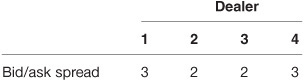
The bid/ask spread as computed above is measured relative to a dealer. The best bid/ask spread is two 32nds for Dealers 2 and 3.
From the perspective of the market overall, the bid/ask spread can be computed by looking at the best bid price (high price at which one of the dealers is willing to buy the security) and the lowest ask price (lowest offer price at which one of the dealers is willing to sell the security). This liquidity measure is called the market bid/ask spread. For the four dealers, the highest bid price is 92 plus two 32nds and the lowest ask price is 92 plus three 32nds. Thus the market bid/ask spread is one 32nd.
For investors who plan to hold a bond until maturity and need not mark a position to market, liquidity risk is not a major concern. An institutional investor who plans to hold an issue to maturity but is periodically marked to market is concerned with liquidity risk. By marking a position to market, it is meant that the security is revalued in the portfolio based on its current market price. For example, mutual funds are required to mark to market at the end of each day the holdings that are in their portfolio in order to compute the net asset value (NAV). While other institutional investors may not mark to market as frequently as mutual funds, they are marked to market when reports are periodically sent to clients or the board of directors or trustees.
Where are the prices obtained to mark a position to market? Typically, a portfolio manager will solicit indicative bids from several dealers and then use some process to determine the bid price used to mark the position. The less liquid the issue, the greater the variation there will be in the bid prices obtained from dealers. With an issue that has little liquidity, the price may have to be determined by a pricing service rather than by dealers. Moreover, lack of dealer indicative bids and concern with models used by pricing services may lead the manager to occasionally override a bid (subject to internal approval beyond the control of the manager).
EXCHANGE-RATE, OR CURRENCY, RISK
A non-dollar-denominated bond (i.e., a bond whose payments occur in a foreign currency) has unknown U.S. dollar cash-flows. The dollar cash-flows are dependent on the foreign-exchange-rate at the time the payments are received. For example, suppose that an investor purchases a bond whose payments are in Japanese yen. If the yen depreciates relative to the U.S. dollar, then fewer dollars will be received. The risk of this occurring is referred to as exchange-rate risk, or currency risk. Of course, should the yen appreciate relative to the U.S. dollar, the investor will benefit by receiving more dollars.
In addition to the change in the exchange-rate, an investor is exposed to the interest-rate, or market, risk in the local market. For example, if a U.S. investor purchases German government bonds denominated in euros, the proceeds received from the sale of that bond prior to maturity will depend on the level of interest rates in the German bond market, in addition to the exchange-rate.
VOLATILITY RISK
As will be explained in later chapters, the price of a bond with an embedded option depends on the level of interest rates and factors that influence the value of the embedded option. One of the factors is the expected volatility of interest rates. Specifically, the value of an option rises when expected interest-rate volatility increases. In the case of a callable bond or mortgage-backed security, because the investor has granted an option to the borrower, the price of the security falls because the investor has given away a more valuable option. The risk that a change in volatility will adversely affect the price of a security is called volatility risk.
Multifactor risk models often refer to volatility risk as vega. This is because in option theory, there are measures of the exposure of an option to changes in the factors that affect an option’s value. One of the factors is volatility, and vega is the term used to measure the sensitivity of an option’s price to a change in volatility. Hence, the sensitivity of bonds with embedded options and a bond portfolio containing bonds with embedded options to changes in volatility is given the same name.
POLITICAL OR LEGAL RISK
Sometimes the government can declare withholding or other additional taxes on a bond or declare a tax-exempt bond taxable. In addition, a regulatory authority can conclude that a given security is unsuitable for investment entities that it regulates. These actions can adversely affect the value of the security. Similarly, it is also possible that a legal or regulatory action affects the value of a security positively. The possibility of any political or legal actions adversely affecting the value of a security is known as political or legal risk.
To illustrate political or legal risk, consider investors who purchase tax-exempt municipal securities. They are exposed to two types of political risk that can be more appropriately called tax risk. The first type of tax risk is that the federal income tax rate will be reduced. The higher the marginal tax rate, the greater is the value of the tax-exempt nature of a municipal security. As the marginal tax rates decline, the price of a tax-exempt municipal security will decline. For example, proposals for a flat tax with a low tax rate significantly reduced the potential tax advantage of owning municipal bonds. As a result, tax-exempt municipal bonds began trading at lower prices. The second type of tax risk is that a municipal bond issued as tax exempt eventually will be declared taxable by the Internal Revenue Service (IRS). This may occur because many municipal (revenue) bonds have elaborate security structures that could be subject to future adverse congressional actions and IRS interpretations. As a result of the loss of the tax exemption, the municipal bond will decline in value in order to provide a yield comparable to similar taxable bonds.
EVENT RISK
Occasionally, the ability of an issuer to make interest and principal payments is seriously and unexpectedly changed by (1) a natural or industrial accident or (2) a takeover or corporate restructuring. These risks are referred to as event risk. The cancellation of plans to build a nuclear power plant illustrates the first type of event in relation to the utility industry.
An example of the second type of event risk is the takeover in 1988 of RJR Nabisco for $25 billion via a financing technique known as a leveraged buyout (LBO). In such a transaction, the new company incurred a substantial amount of debt to finance the acquisition of the firm. Because the corporation was required to service a substantially larger amount of debt, its quality rating was reduced to non-investment-grade quality. As a result, the change in yield spread to a benchmark Treasury, demanded by investors because of the LBO announcement, increased from about 100 to 350 basis points.
There are also spillover effects of event risk on other firms. For example, if there is a nuclear accident, this will affect all utilities producing nuclear power.
SECTOR RISK
Bonds in different sectors of the market respond differently to environmental changes because of a combination of some or all of the preceding risks, as well as others. Examples include discount versus premium coupon bonds, industrial versus utility bonds, and corporate versus mortgage-backed bonds. The possibility of adverse differential movement of specific sectors of the market is called sector risk.
OTHER RISKS
The various risks of investing in the fixed income markets reviewed in this chapter do not represent the entire range of risks. In the marketplace, it is customary to combine almost all risks other than market risk (interest-rate risk) and refer to it as basis risk.
STATISTICAL MEASURES OF PORTFOLIO RISK: STANDARD DEVIATION, SKEWNESS, AND KURTOSIS
In the development of portfolio theory as formulated by Harry Markowitz (also known as mean-variance analysis), a portfolio’s risk is measured by the standard deviation of historical portfolio returns.4 This statistical measure provides a range around the average return of a portfolio within which the actual return over a period is likely to fall with some specific probability. In evaluating actual and potential performance relative to a benchmark that is a bond index, the mean return and standard deviation of returns of the bond index and the portfolio are compared.
Extensions of portfolio risk to take into account other statistical measures of a return distribution are being used in practice.5 Two statistical measures most commonly used are skewness and kurtosis. A return distribution is said to be symmetric based on the probability distribution around the mean or expected value. If the return distribution is the same above and below the mean value, then the distribution is said to be symmetric. If a return distribution does not exhibit this property, it is said to be asymmetric. Skewness is a measure of the symmetry of a return distribution. Actually, it is more meaningful to say that skewness is a measure of the lack of symmetry of the return distribution. The normal distribution is a symmetric distribution. Consequently, when the return distribution is assumed to be normally distributed, skewness is not a concern.
Kurtosis is a statistical measure of whether a return distribution is peaked or flat relative to a normal distribution. That is, a return distribution with high kurtosis tends to have a distinct peak near the mean value, decline rather rapidly, and has fat (or heavy) tails. This property for a return distribution occurs when in addition to many modest-sized deviations from the mean value there are also infrequent extreme deviations from the mean value. Return distributions that exhibit low kurtosis tend to have a flat top near the mean value rather than a sharp peak.
TRACKING ERROR RISK
A bond portfolio’s standard deviation and a designated benchmark’s standard deviation are absolute numbers. A portfolio manager can compare the mean values and standard deviations to try to get a feel for the risk profile of the portfolio relative to the benchmark. If skewness and kurtosis are also considered, this would provide an expanded profile of the relative risks of the bond portfolio and the bond index.
A portfolio manager or client can also assess what the variation in the portfolio’s return is relative to a benchmark (such as a bond index) by looking at the deviations of the periodic (weekly or monthly) portfolio return from that of the benchmark. The difference between the two is called the active return. That is
Active return = Portfolio’s actual return – Benchmark’s actual return
From the active returns, a portfolio’s risk relative to the benchmark can be calculated by the standard deviation of the active returns. This standard deviation is referred to as tracking error risk or tracking error volatility, or simply tracking error.
The larger a portfolio’s tracking error, the more its risk profile deviates from that of the benchmark. In fact, when bond portfolio strategies are discussed in later chapters, we will see that there are active and passive strategies. The latter strategies involve little tracking error. For example, a portfolio constructed to match the performance of a bond index will have a tracking error close to zero. Active strategies will have higher tracking error, how much higher depending on the degree of risk the portfolio manager or client is willing to accept.
There are two types of tracking error. Tracking error calculated from a portfolio’s historical active returns is called backward-looking tracking error. It is also called historical tracking error and ex-post tracking error. The limitation of backward-looking tracking error is that it fails to take into account the effect of current decisions by the portfolio manager on the future active returns and therefore may have little predictive value and can be misleading regarding the portfolio risks going forward. The other type of tracking error is forward-looking tracking error—also called predicted tracking error and ex-ante tracking error. This form of tracking error seeks to accurately reflect the portfolio’s risk going forward. In practice, forward-looking tracking error is estimated using a multi-factor risk model as described in Chapters 46 and 47.
KEY POINTS
• The risks associated with investing in individual fixed income securities are interest-rate risk, reinvestment risk, call/prepayment risk, credit risk, inflation (or purchasing-power) risk, liquidity risk, exchange-rate (or currency) risk, volatility risk, political or legal risk, event risk, and sector risk.
• Interest-rate risk is the risk associated with an adverse change in interest rates and includes level risk and yield-curve risk. The most popular measure of level risk is duration; key rate duration is the most popular measure of yield-curve risk.
• Credit risk includes default risk, credit-spread risk, and downgrade risk. Credit risk models seek to estimate the probability distribution of losses for a bond portfolio.
• Portfolio risk measures include statistical measures of return and tracking error risk.
• Statistical measures of portfolio and benchmark risk include the standard deviation, skewness, and kurtosis.
• Tracking error risk is the standard deviation of the active return of a portfolio (i.e., the difference between the portfolio’s return and the benchmark’s return). Backward-looking tracking error is used to assess a portfolio’s performance relative to a benchmark. Forward-looking tracking error is used to predict future performance relative to a benchmark.