CHAPTER
SEVEN
MEASURING INTEREST-RATE RISK

FRANK J. FABOZZI, PH.D., CFA, CPA

Professor of Finance
EDHEC Business School

GERALD W. BUETOW, JR., PH.D., CFA

Chief Investment Officer
Innealta Capital

ROBERT R. JOHNSON, PH.D., CFA

Senior Managing Director
CFA Institute

BRIAN J. HENDERSON, PH.D., CFA

Assistant Professor
The George Washington University

The value of a bond changes in the opposite direction of the change in interest rates. A long bond position’s value will decline if interest rates rise, resulting in a loss. For a short bond position, a loss will be realized if interest rates fall. However, an investor wants to know more than simply when a position will realize a loss. To control interest-rate risk, an investor must be able to quantify what will result.

The key to measuring interest-rate risk is the accuracy of the estimate of the value of the position after an adverse rate change. A valuation model is used to determine the value of a position after an adverse rate move. Consequently, if a reliable valuation model is not used, there is no way to properly measure interest-rate risk exposure.

There are two approaches to measuring interest-rate risk—the full-valuation approach and the duration/convexity approach. We begin with a discussion of the full-valuation approach. The balance of the chapter is devoted to the duration/convexity approach. As a background to the duration/convexity approach, we discuss the price volatility characteristics of option-free bonds and bonds with embedded options. We then look at how duration can be used to estimate interest-rate risk and distinguish between various duration measures (effective, modified, and Macaulay). Next, we show how a measure referred to as “convexity” can be used to improve the duration estimate of the price volatility of a bond to rate changes. In the next to the last section we show the relationship between duration and another measure of price volatility used by investors, the price value of a basis point (or dollar value of an 01). In the last section we discuss the importance of incorporating yield volatility in estimates of exposure to interest-rate risk.

Parts of this chapter are adapted from several chapters in Frank J. Fabozzi, Duration, Convexity, and Other Bond Risk Measures (New Hope, PA: Frank J. Fabozzi Associates, 1999) and from Gerald W. Buetow and Robert R. Johnson, “A Primer on Effective Duration and Convexity,” in Frank J. Fabozzi (ed.), Professional Perspectives on Fixed Income Portfolio Management, Vol. 1 (New Hope, PA: Frank J. Fabozzi Associates, 2000).

THE FULL-VALUATION APPROACH

The most obvious way to measure the interest-rate risk exposure of a bond position or a portfolio is to revalue it when interest rates change. The analysis is performed for a given scenario with respect to interest-rate changes. For example, an investor may want to measure the interest-rate exposure to a 50 basis point, 100 basis point, and 200 basis point instantaneous change in interest rates. This approach requires the revaluation of a bond or bond portfolio for a given interest-rate change scenario and is called the full-valuation approach. It is sometimes referred to as “scenario analysis” because it involves assessing the exposure to interest-rate change scenarios.

To illustrate this approach, suppose that an investor has a $10 million par value position in a 5% coupon 20-year bond. The bond is option-free. The current price is 106.5484 for a yield (i.e., yield to maturity) of 4.5%. The market value of the position is $10,654,840 (106.5484% × $10 million). Since the investor owns the bond, she is concerned with a rise in yield, since this will decrease the market value of the position. To assess the exposure to a rise in market yields, the investor decides to look at how the value of the bond will change if yields change instantaneously for the following three scenarios: (1) 50 basis point increase, (2) 100 basis point increase, and (3) 200 basis point increase. This means that the investor wants to assess what will happen to the bond position if the yield on the bond increases from 4.5% to (1) 5%, (2) 5.5%, and (3) 6.5%. Because this is an option-free bond, valuation is straightforward. We will assume that one yield is used to discount each of the cash-flows. That is, we will assume a flat yield-curve. The price of this bond per $100 par value and the market value of the $10 million par position is shown in Exhibit 7–1. Also shown is the change in the market value and the percentage change.

EXHIBIT 7–1
Illustration of Full-Valuation Approach to Assess the Interest-Rate Risk of a Bond Position for Three Scenarios

In the case of a portfolio, each bond is valued for a given scenario, and then the total value of the portfolio is computed for the scenario. For example, suppose that a manager has a portfolio with the following two option-free bonds: (1) 4% coupon 5-year bond and (2) 5% coupon 20-year bond. For the shorter-term bond, $5 million of par value is owned, and the price is 109.4713 for a yield of 2%. For the longer-term bond, $10 million of par value is owned, and the price is 106.5484 for a yield of 4.5%. Suppose that the manager wants to assess the interest-rate risk of this portfolio for a 50, 100, and 200 basis point increase in interest rates assuming that both the 5-year yield and the 20-year yield change by the same number of basis points. Exhibit 7–2 shows the exposure. Panel a of the exhibit shows the market value of the 5-year bond for the three scenarios. Panel b does the same for the 20-year bond. Panel c shows the total market value of the portfolio and the percentage change in the market value for the three scenarios.

In Exhibit 7–2, it is assumed that both the 5-year and the 20-year yields changed by the same number of basis points. The full-valuation approach also can handle scenarios where the yield-curve does not change in a parallel fashion. Exhibit 7–3 illustrates this for our portfolio that includes the 5-year and the 20-year bonds. The scenario analyzed is a yield-curve shift scenario combined with scenarios for shifts in the level of yields. In the illustration in Exhibit 7–3, the following yield changes for the 5-year and 20-year yields are assumed:

EXHIBIT 7–2
Illustration of Full-Valuation Approach to Assess the Interest-Rate Risk of a Bond Portfolio for Three Scenarios Assuming a Parallel Shift in the Yield-Curve

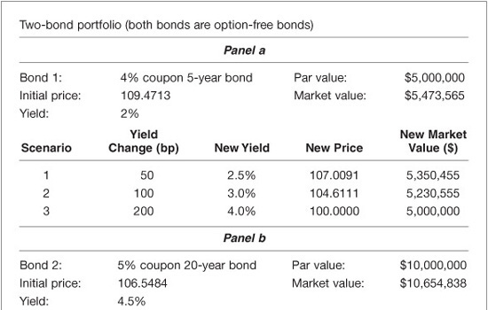
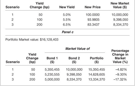
EXHIBIT 7–3
Illustration of Full-Valuation Approach to Assess the Interest-Rate Risk of a Bond Portfolio for Three Scenarios Assuming a Nonparallel Shift in the Yield-Curve

The last panel in Exhibit 7–3 shows how the market value of the portfolio changes for each scenario.

The full-valuation approach seems straightforward. If one has a good valuation model, assessing how the value of a portfolio or individual bond will change for different scenarios for parallel and nonparallel yield-curve shifts measures the interest-rate risk of a portfolio.

A common question that often arises when using the full-valuation approach is what scenarios should be evaluated to assess interest-rate risk exposure. For some regulated entities, there are specified scenarios established by regulators. For example, it is common for regulators of depository institutions to require entities to determine the impact on the value of their bond portfolio for a 100, 200, and 300 basis point instantaneous change in interest rates (up and down). (Regulators tend to refer to this as “simulating” interest-rate scenarios rather than scenario analysis.) Risk managers and highly leveraged investors such as hedge funds tend to look at extreme scenarios to assess exposure to interest-rate changes. This practice is called stress testing.

Of course, in assessing how changes in the yield-curve can affect the exposure of a portfolio, there are an infinite number of scenarios that can be evaluated. The state-of-the-art technology involves using a complex statistical procedure to determine a likely set of yield-curve shift scenarios from historical data.

We can use the full-valuation approach to assess the exposure of a bond or portfolio to interest-rate change to evaluate any scenario, assuming—and this must be repeated continuously—that the investor has a good valuation model to estimate what the price of the bonds will be in each interest-rate scenario. While the full-valuation approach is the recommended approach for assessing the position of a single bond or a portfolio of a few bonds, for a portfolio with a large number of bonds and with even a minority of those bonds being complex (i.e., having embedded options), the full-valuation process is time-consuming. Investors want one measure they can use to get an idea of how a portfolio or even a single bond will change if rates change in a parallel fashion rather than having to revalue a portfolio to obtain that answer. Such a measure is duration. We will discuss this measure as well as a supplementary measure (convexity). To build a foundation to understand the limitations of these measures, we describe next the basic price volatility characteristics of bonds. The fact that there are limitations of using one or two measures to describe the interest-rate exposure of a position or portfolio should not be surprising. What is important to understand is that these measures provide a starting point for assessing interest-rate risk.

PRICE VOLATILITY CHARACTERISTICS OF BONDS

The characteristics of a bond that affect its price volatility are (1) maturity, (2) coupon rate, and (3) presence of embedded options. We also will see how the level of yields affects price volatility.

Price Volatility Characteristics of Option-Free Bonds

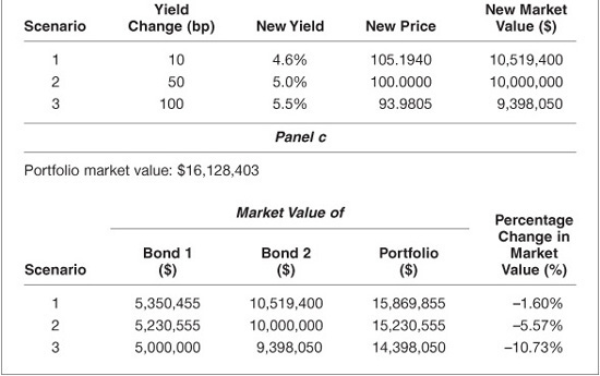
We begin by focusing on option-free bonds (i.e., bonds that do not have embedded options). A fundamental characteristic of an option-free bond is that the price of the bond changes in the opposite direction from a change in the bond’s required yield. Exhibit 7–4 illustrates this property for four hypothetical bonds assuming a par value of $100.

EXHIBIT 7–4
Price/Yield Relationship for Four Hypothetical Option-Free Bonds

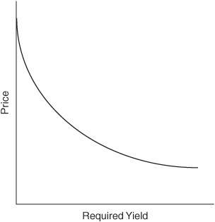
When the price/yield relationship for any option-free bond is graphed, it exhibits the shape shown in Exhibit 7–5. Notice that as the required yield increases, the price of an option-free bond declines. However, this relationship is not linear (i.e., not a straight-line relationship). The shape of the price/yield relationship for any option-free bond is called convex. This price/yield relationship is for an instantaneous change in the required yield.

EXHIBIT 7–5
Price/Yield Relationship for a Hypothetical Option-Free Bond

The price sensitivity of a bond to changes in the required yield can be measured in terms of the dollar price change or the percentage price change. Exhibit 7–6 uses the four hypothetical bonds in Exhibit 7–4 to show the percentage change in each bond’s price for various changes in yield, assuming that the initial yield for all four bonds is 4%. An examination of Exhibit 7–6 reveals the following properties concerning the price volatility of an option-free bond:

EXHIBIT 7–6
Instantaneous Percentage Price Change for Four Hypothetical Bonds (Initial yield for all four bonds is 4%)

Property 1: Although the price moves in the opposite direction from the change in required yield, the percentage price change is not the same for all bonds.

Property 2: For small changes in the required yield, the percentage price change for a given bond is roughly the same, whether the required yield increases or decreases.

Property 3: For large changes in required yield, the percentage price change is not the same for an increase in required yield as it is for a decrease in required yield.

Property 4: For a given large change in basis points in the required yield, the percentage price increase is greater than the percentage price decrease.

While the properties are expressed in terms of percentage price change, they also hold for dollar price changes.

The implication of Property 4 is that if an investor is long a bond, the price appreciation that will be realized if the required yield decreases is greater than the capital loss that will be realized if the required yield increases by the same number of basis points. For an investor who is short a bond, the reverse is true: The potential capital loss is greater than the potential capital gain if the yield changes by a given number of basis points.

Bond Features That Affect Interest-Rate Risk

The degree of sensitivity of a bond’s price to changes in market interest rates (i.e., a bond’s interest-rate risk) depends on various features of the issue, such as maturity, coupon rate, and embedded options.

The Impact of Maturity

All other factors constant, the longer the bond’s maturity, the greater is the bond’s price sensitivity to changes in interest rates. For example, for a 4% 20-year bond selling to yield 4%, a rise in the yield required by investors to 4.5% will cause the bond’s price to decline from 100 to 93.4516, a 6.55% price decline. For a 4% 5-year bond selling to yield 4%, the price is 100. A rise in the yield required by investors from 4% to 4.5% would decrease the price to 97.7834. The decline in the bond’s price is only 2.22%.

The Impact of Coupon Rate

A property of a bond is that all other factors constant, the lower the coupon rate, the greater is the bond’s price sensitivity to changes in interest rates. For example, consider a 5% 20-year bond selling to yield 4%. The price of this bond would be 113.6777. If the yield required by investors increases by 50 basis points to 4.5%, the price of this bond would fall by 6.27% to 106.5484. This decline is less than the 6.55% decline for the 4% 20-year bond selling to yield 4%.

An implication is that zero-coupon bonds have greater price sensitivity to interest-rate changes than same-maturity bonds bearing a coupon rate and trading at the same yield.

The Impact of Embedded Options

In Chapter 1 the various embedded options that may be included in a bond issue were discussed. The value of a bond with embedded options will change depending on how the value of the embedded options changes when interest rates change. For example, as interest rates decline, the price of a callable bond may not increase as much as an otherwise option-free bond (i.e., a bond with no embedded options).

To understand why, we decompose the price of a callable bond into two parts, as shown below:

Price of callable bond

= price of option-free bond – price of embedded call option

The reason for subtracting the price of the embedded call option from the price of the option-free bond is that the call option is a benefit to the issuer and a disadvantage to the bondholder. This reduces the price of a callable bond relative to an option-free bond.

Now, when interest rates decline, the price of an option-free bond increases. However, the price of the embedded call option increases when interest rates decline because the call option becomes more valuable to the issuer. Thus, when interest rates decline, both components increase, but the change in the price of the callable bond depends on the relative price change of the two components. Typically, a decline in interest rates will result in an increase in the price of the callable bond but not by as much as the price change of an otherwise comparable option-free bond.

Similarly, when interest rates rise, the price of a callable bond will not fall by as much as an otherwise option-free bond. The reason is that the price of the embedded call option declines. When interest rates rise, the price of the option-free bond declines but is partially offset by the decrease in the price of the embedded call option.

Price Volatility Characteristics of Bonds with Embedded Options

In this section we examine the price/yield relationship for bonds with both types of options (calls and puts) and implications for price volatility.

Bonds with Call and Prepay Options

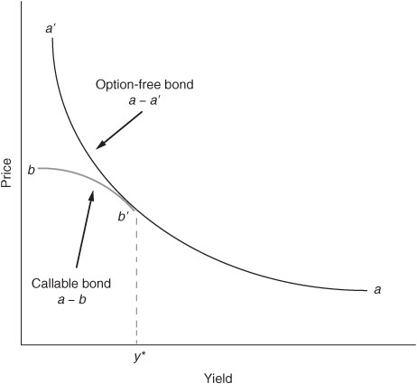
In the discussion below we will refer to a bond that may be called or is prepayable as a callable bond. Exhibit 7–7 shows the price/yield relationship for an option-free bond and a callable bond. The convex curve given by a–a´ is the price/yield relationship for an option-free bond. The unusually shaped curve denoted by a–b in the exhibit is the price/yield relationship for the callable bond.

EXHIBIT 7–7
Price/Yield Relationship for a Callable Bond and an Option-Free Bond

The reason for the price/yield relationship for a callable bond is as follows. When the prevailing market yield for comparable bonds is higher than the coupon rate on the callable bond, it is unlikely that the issuer will call the issue. For example, if the coupon rate on a bond is 3% and the prevailing market yield on comparable bonds is 6%, it is highly unlikely that the issuer will call a 3% coupon bond so that it can issue a 6% coupon bond. Since the bond is unlikely to be called, the callable bond will have a similar price/yield relationship as an otherwise comparable option-free bond. Consequently, the callable bond is going to be valued as if it is an option-free bond. However, since there is still some value to the call option, the bond won’t trade exactly like an option-free bond.

As yields in the market decline, the concern is that the issuer will call the bond. The issuer won’t necessarily exercise the call option as soon as the market yield drops below the coupon rate. Yet the value of the embedded call option increases as yields approach the coupon rate from higher yield levels. For example, if the coupon rate on a bond is 3% and the market yield declines to 3.50%, the issuer most likely will not call the issue. However, market yields are at a level at which the investor is concerned that the issue eventually may be called if market yields decline further. Cast in terms of the value of the embedded call option, that option becomes more valuable to the issuer, and therefore, it reduces the price relative to an otherwise comparable option-free bond.¹ In Exhibit 7–7, the value of the embedded call option at a given yield can be measured by the difference between the price of an option-free bond (the price shown on the curve a–a´) and the price on the curve a–b. Notice that at low yield levels (below y^* on the horizontal axis), the value of the embedded call option is high.

Let’s look at the difference in the price volatility properties relative to an option-free bond given the price/yield relationship for a callable bond shown in Exhibit 7–7. Exhibit 7–8 blows up the portion of the price/yield relationship for the callable bond where the two curves in Exhibit 7–7 depart (segment b–b´ in Exhibit 7–7). We know from our discussion of the price/yield relationship that for a large change in yield of a given number of basis points, the price of an option-free bond increases by more than it decreases (Property 4 discussed previously). Is that what happens for a callable bond in the region of the price/yield relationship shown in Exhibit 7–8? No, it is not. In fact, as can be seen in the exhibit, the opposite is true! That is, for a given large change in yield, the price appreciation is less than the price decline.

EXHIBIT 7–8
Negative Convexity Region of the Price/Yield Relationship for a Callable Bond

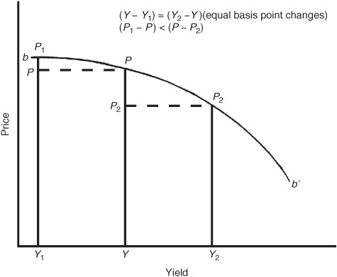
The price volatility characteristic of a callable bond is important to understand. The characteristic of a callable bond that its price appreciation is less than its price decline when rates change by a large number of basis points is called negative convexity.² But notice from Exhibit 7–7 that callable bonds do not exhibit this characteristic at every yield level. When yields are high (relative to the issue’s coupon rate), the bond exhibits the same price/yield relationship as an option-free bond and therefore at high-yield levels also has the characteristic that the gain is greater than the loss. Because market participants have referred to the shape of the price/yield relationship shown in Exhibit 7–8 as negative convexity, market participants call the relationship for an option-free bond positive convexity. Consequently, a callable bond exhibits negative convexity at low yield levels and positive convexity at high-yield levels.

As can be seen from the exhibits, when a bond exhibits negative convexity, as rates decline, the bond compresses in price. That is, at a certain yield level there is very little price appreciation when rates decline. When a bond enters this region, the bond is said to exhibit “price compression.”

Bonds with Embedded Put Options

Putable bonds may be redeemed by the bondholder on the dates and at the put price specified in the indenture. Typically, the put price is par value. The advantage to the investor is that if yields rise such that the bond’s value falls below the put price, the investor will exercise the put option. If the put price is par value, this means that if market yields rise above the coupon rate, the bond’s value will fall below par, and the investor will then exercise the put option.

The value of a putable bond is equal to the value of an option-free bond plus the value of the put option. Thus the difference between the value of a putable bond and the value of an otherwise comparable option-free bond is the value of the embedded put option. This can be seen in Exhibit 7–9 which shows the price/yield relationship for a putable bond (the curve a´–b) and an option-free bond (the curve a´–a´).

EXHIBIT 7–9
Price/Yield Relationship for a Putable Bond and an Option-Free Bond

At low yield levels (low relative to the issue’s coupon rate), the price of the putable bond is basically the same as the price of the option-free bond because the value of the put option is small. As rates rise, the price of the putable bond declines, but the price decline is less than that for an option-free bond. The divergence in the price of the putable bond and an otherwise comparable option-free bond at a given yield level is the value of the put option. When yields rise to a level where the bond’s price would fall below the put price, the price at these levels is the put price.

Interest-Rate Risk for Floating-Rate Securities

The change in the price of a fixed-rate coupon bond when market interest rates change is due to the fact that the bond’s coupon rate differs from the prevailing market interest rate. For a floating-rate security, the coupon rate is reset periodically based on the prevailing value for the reference rate plus the quoted margin. The quoted margin is set for the life of the security. The price of a floating-rate security will fluctuate depending on three factors.

First, the longer the time to the next coupon reset date, the greater is the potential price fluctuation.³ For example, consider a floating-rate security whose coupon resets every six months and the coupon formula is the six-month Treasury rate plus 20 basis points. Suppose that on the coupon reset date the six-month Treasury rate is 0.35%. If on the day after the coupon is reset the six-month Treasury rate rises to 0.75%, this means that this security is offering a six-month coupon rate that is less than the prevailing six-month rate for the remaining six months. The price of the security must decline to reflect this. Suppose instead that the coupon resets every month at the one-month Treasury rate and that this rate rises immediately after the coupon rate is reset. In this case, while the investor would be realizing a submarket one-month coupon rate, it is for only a month. The price decline will be less than for the security that resets every six months.

The second reason why a floating-rate security’s price will fluctuate is that the required margin that investors demand in the market changes. For example, consider once again the security whose coupon formula is the six-month Treasury rate plus 20 basis points. If market conditions change such that investors want a margin of 30 basis points rather than 20 basis points, this security would be offering a coupon rate that is 10 basis points below the market rate. As a result, the security’s price will decline.

Finally, a floating-rate security typically will have a cap. Once the coupon rate as specified by the coupon formula rises above the cap rate, the coupon will be set at the cap rate, and the security then will offer a below-market coupon rate, and its price will decline. In fact, once the cap is reached, the security’s price will react much the same way to changes in market interest rates as that of a fixed-rate coupon security. This risk for a floating-rate security is called cap risk.

The Impact of the Yield Level

Because of credit risk, different bonds trade at different yields, even if they have the same coupon rate, maturity, and embedded options. How, then, holding other factors constant, does the level of interest rates affect a bond’s price sensitivity to changes in interest rates? As it turns out, the higher the level of interest rates that a bond trades, the lower is the price sensitivity.

To see this, we can compare a 5% 20-year bond initially selling at a yield of 5% and a 5% 20-year bond initially selling at a yield of 9%. The former is initially at a price of 100, and the latter, 63.20. Now, if the yield on both bonds increases by 100 basis points, the first bond trades down by 11.56 points (11.56%) to a price of 88.44. After the assumed increase in yield, the second bond will trade at a price of 57.10, for a price decline of only 6.09 points (or 9.64%). Thus we see that the bond that trades at a lower yield is more volatile in both percentage price change and absolute price change as long as the other bond characteristics are the same. An implication is that for a given change in interest rates, price sensitivity is lower when the level of interest rates in the market is high, and price sensitivity is higher when the level of interest rates is low.

DURATION

With this background about the price volatility characteristics of a bond, we can now turn to an alternate approach to full valuation: the duration/convexity approach. Duration is a measure of the approximate sensitivity of a bond’s value to rate changes. More specifically, it is the approximate percentage change in value for a 100 basis point change in rates. We’ll see in this section that duration is the first approximation of the percentage price change. To improve the estimate provided by duration a measure called convexity can be used. Hence, using duration combined with convexity to estimate the percentage price change of a bond to changes in interest rates is called the duration/convexity approach.

Calculating Duration

The duration of a bond is estimated as follows:

If we let

y = change in yield in decimal

V₀ = initial price

V₋ = price if yields decline by

V₊ = price if yields increase by y

then duration can be expressed as

For example, consider a 5% coupon 20-year option-free bond selling at 113.6777 to yield 4% (see Exhibit 7–4). Let’s change (i.e., shock) the yield down and up by 20 basis points and determine what the new prices will be for the numerator. If the yield is decreased by 20 basis points from 4.0% to 3.8%, the price would increase to 116.7049. If the yield increases by 20 basis points, the price would decrease to 110.7527. Thus

y = 0.002

V₀ = 113.6777

V₋ = 116.7049

V₊ = 110.5727

Then

Duration is interpreted as the approximate percentage change in price for a 100 basis point change in rates. Consequently, a duration of 13.09 means that the approximate change in price for this bond is 13.09% for a 100 basis point change in rates.

A common question asked about this interpretation of duration is the consistency between the yield change that is used to compute duration using Eq. (7–1) and the interpretation of duration. For example, recall that in computing the duration of the 5% coupon 20-year bond, we used a 20 basis point yield change to obtain the two prices to use in the numerator of Eq. (7–1). Yet we interpret the duration computed as the approximate percentage price change for a 100 basis point change in yield. The reason is that regardless of the yield change used to estimate duration in Eq. (7–1), the interpretation is the same. If we used a 25 basis point change in yield to compute the prices used in the numerator of Eq. (7–1), the resulting duration is interpreted as the approximate percentage price change for a 100 basis point change in yield. Later we will use different changes in yield to illustrate the sensitivity of the computed duration.

Approximating the Percentage Price Change Using Duration

The following formula is used to approximate the percentage price change for a given change in yield and a given duration:

The reason for the negative sign on the right-hand side of Eq. (7–2) is due to the inverse relationship between price change and yield change.

For example, consider the 5% 20-year bond trading at 113.6777 whose duration we just showed is 13.09. The approximate percentage price change for a 10 basis point increase in yield (i.e., y = +0.001) is

Approximate percentage price change = –13.09 × (+0.001) × 100 = −1.309%

How good is this approximation? The actual percentage price change is –1.30% (as shown in Exhibit 7–6 when yield increases to 4.10%). Duration, in this case, did an excellent job in estimating the percentage price change. We would come to the same conclusion if we used duration to estimate the percentage price change if the yield declined by 10 basis points (i.e., y = –0.001). In this case, the approximate percentage price change would be +1.309% (i.e., the direction of the estimated price change is the reverse but the magnitude of the change is the same). Exhibit 7–6 shows that the actual percentage price change is +1.32%.

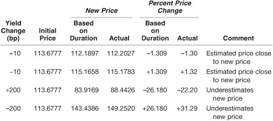
In terms of estimating the new price, let’s see how duration performed. The initial price is 113.6777. For a 10 basis point increase in yield, duration estimates that the price will decline by 1.309%. Thus the price will decline to 112.1897 (found by multiplying 113.6777 by 1 minus 0.01309). The actual price from Exhibit 7–4 if the yield increases by 10 basis points is 112.2027. Thus the price estimated using duration is close to the actual price. For a 10 basis point decrease in yield, the actual price from Exhibit 7–4 is 115.1783, and the estimated price using duration is 115.1658 (a price increase of 1.309%). Consequently, the new price estimated by duration is close to the actual price for a 10 basis point change in yield.

Let’s look at how well duration does in estimating the percentage price change if the yield increases by 200 basis points instead of 10 basis points. In this case, y is equal to +0.02. Substituting into Eq. (7–2) we have

Approximate percentage price change = −13.09 × (+0.02) × 100 = −26.18%

How good is this estimate? From Exhibit 7–6 we see that the actual percentage price change when the yield increases by 200 basis points to 6% is –22.20%. Thus the estimate is not as accurate as when we used duration to approximate the percentage price change for a change in yield of only 10 basis points. If we use duration to approximate the percentage price change when the yield decreases by 200 basis points, the approximate percentage price change in this scenario is +26.18%. The actual percentage price change as shown in Exhibit 7–6 is +31.29%.

Again, let’s look at the use of duration in terms of estimating the new price. Since the initial price is 113.6777 and a 200 basis point increase in yield will decrease the price by 26.18%, the estimated new price using duration is 83.9169 (found by multiplying 113.6777 by 1 minus 0.2618). From Exhibit 7–4 the actual price if the yield is 6% is 88.4426. Consequently, the estimate is not as accurate as the estimate for a 10 basis point change in yield. The estimated new price using duration for a 200 basis point decrease in yield is 143.4386 compared with the actual price (from Exhibit 7–4) of 149.2520. Once again, the estimation of the price using duration is not as accurate as for a 10 basis point change. Notice that whether the yield is increased or decreased by 200 basis points, duration underestimates what the new price will be. We will see why shortly.

Let’s summarize what we found in our application of duration to approximate the percentage price change:

Look again at Eq. (7–2). Notice that whether the change in yield is an increase or a decrease, the approximate percentage price change will be the same except that the sign is reversed. This violates Properties 3 and 4 with respect to the price volatility of option-free bonds when yields change. Recall that Property 3 states that the percentage price change will not be the same for a large increase and decrease in yield by the same number of basis points. This is one reason why we see that the estimate is inaccurate for a 200 basis point yield change. Why did the duration estimate of the price change do a good job for a small change in yield of 10 basis points? Recall from Property 2 that the percentage price change will be approximately the same whether there is an increase or decrease in yield by a small number of basis points. We also can explain these results in terms of the graph of the price/yield relationship. We will do this next.

Graphic Depiction of Using Duration to Estimate Price Changes

The shape of the price/yield relationship for an option-free bond is convex. Exhibit 7–10 shows this relationship. In the exhibit, a tangent line is drawn to the price/yield relationship at yield y^*. [For those unfamiliar with the concept of a tangent line, it is a straight line that just touches a curve at one point within a relevant (local) range.] In Exhibit 7–10, the tangent line touches the curve at the point where the yield is equal to y^* and the price is equal to p^*. The tangent line can be used to estimate the new price if the yield changes. If we draw a vertical line from any yield (on the horizontal axis), as in Exhibit 7–10, the distance between the horizontal axis and the tangent line represents the price approximated by using duration starting with the initial yield y^*.

EXHIBIT 7–10
Price/Yield Relationship for an Option-Free Bond with a Tangent Line

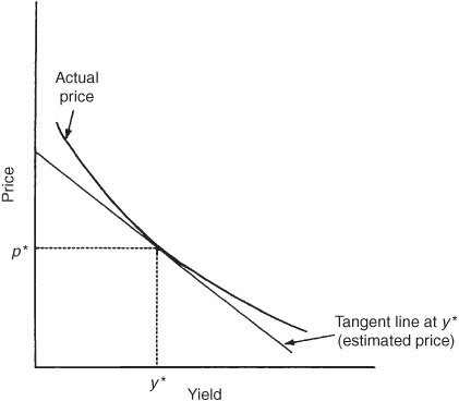
Now how is the tangent line, used to approximate what the new price will be if yields change, related to duration? Duration tells us the approximate percentage price change. Given the initial price and the approximate percentage price change provided by duration [i.e., as given by Eq. (7–2)], the approximate new price can be estimated. Mathematically, it can be demonstrated that the estimated price that is provided by duration is on the tangent line.

This helps us to understand why duration did an effective job of estimating the percentage price change or, equivalently, the new price when the yield changes by a small number of basis points. Look at Exhibit 7–11. Notice that for a small change in yield, the tangent line does not depart much from the price/yield relationship. Hence, when the yield changes up or down by 10 basis points, the tangent line does a good job of estimating the new price, as we found in our earlier numerical illustration.

EXHIBIT 7–11
Estimating the New Price Using a Tangent Line

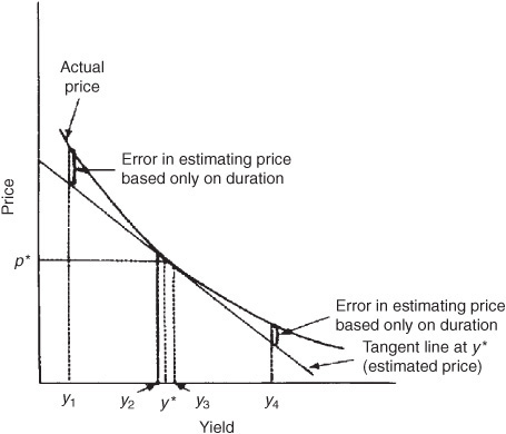
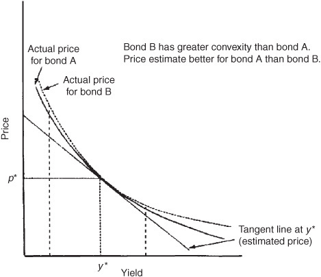
Exhibit 7–11 also shows what happens to the estimate using the tangent line when the yield changes by a large number of basis points. Notice that the error in the estimate gets larger the further one moves from the initial yield. The estimate is less accurate the more convex the bond. This is illustrated in Exhibit 7–12.

EXHIBIT 7–12
Estimating the New Price for a Large Yield Change for Bonds with Different Convexities

Also note that regardless of the magnitude of the yield change, the tangent line always underestimates what the new price will be for an option-free bond because the tangent line is below the price/yield relationship. This explains why we found in our illustration that when using duration we underestimated what the actual price will be.

Rate Shocks and Duration Estimate

In calculating duration using Eq. (7–1), it is necessary to shock interest rates (yields) up and down by the same number of basis points to obtain the values for V₋ and V₊. In our illustration, 20 basis points was arbitrarily selected. But how large should the shock be? That is, how many basis points should be used to shock the rate?

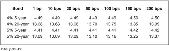
In Exhibit 7–13, the duration estimate for our four hypothetical bonds using Eq. (7–1) for rate shocks of 1 basis point to 200 basis points is reported. The duration estimates for the two 5-year bonds are not affected by the size of the shock. The two 5-year bonds are less convex than the two 20-year bonds. But even for the two 20-year bonds, for the size of the shocks reported in Exhibit 7–13, the duration estimates are not materially affected by the greater convexity.

EXHIBIT 7–13
Duration Estimates for Different Rate Shocks

Thus it would seem that the size of the shock is unimportant. However, the results reported in Exhibit 7–13 are for option-free bonds. When we deal with more complicated securities, small rate shocks that do not reflect the types of rate changes that may occur in the market do not permit the determination of how prices can change because expected cash-flows may change when dealing with bonds with embedded options. In comparison, if large rate shocks are used, we encounter the asymmetry caused by convexity. Moreover, large rate shocks may cause dramatic changes in the expected cash-flows for bonds with embedded options that may be far different from how the expected cash-flows will change for smaller rate shocks.

There is another potential problem with using small rate shocks for complicated securities. The prices that are inserted into the duration formula as given by Eq. (7–1) are derived from a valuation model. In Chapters 40 and 41 we will discuss various valuation models and their underlying assumptions. The duration measure depends crucially on a valuation model. If the rate shock is small and the valuation model used to obtain the prices for Eq. (7–1) is poor, dividing poor price estimates by a small shock in rates in the denominator will have a significant effect on the duration estimate.

What is done in practice by dealers and vendors of analytical systems? Each system developer uses rate shocks he or she believes to be realistic based on historical rate changes.

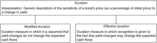
MODIFIED DURATION VERSUS EFFECTIVE DURATION

One form of duration that is cited by practitioners is modified duration. Modified duration is the approximate percentage change in a bond’s price for a 100 basis point change in yield assuming that the bond’s expected cash-flows do not change when the yield changes. What this means is that in calculating the values of V₋ and V₊ in Eq. (7–1), the same cash-flows used to calculate V₀ are used. Therefore, the change in the bond’s price when the yield is changed is due solely to discounting cash-flows at the new yield level.

The assumption that the cash-flows will not change when the yield is changed makes sense for option-free bonds such as noncallable Treasury securities. This is so because the payments made by the U.S. Department of the Treasury to holders of its obligations do not change when interest rates change. However, the same cannot be said for bonds with embedded options (i.e., callable and putable bonds and mortgage-backed securities). For these securities, a change in yield may alter the expected cash-flows significantly.

Earlier we showed the price/yield relationship for callable and prepayable bonds. Failure to recognize how changes in yield can alter the expected cash-flows will produce two values used in the numerator of Eq. (7–1) that are not good estimates of how the price actually will change. The duration is then not a good number to use to estimate how the price will change.

In later chapters where valuation models for bonds with embedded options will be discussed, it will be explained how these models take into account how changes in yield will affect the expected cash-flows. Thus, when V₋ and V₊ are the values produced from these valuation models, the resulting duration takes into account both the discounting at different interest rates and how the expected cash-flows may change. When duration is calculated in this manner, it is called effective duration or option-adjusted duration. Exhibit 7–14 summarizes the distinction between modified duration and effective duration.

EXHIBIT 7–14
Modified Duration versus Effective Duration

The difference between modified duration and effective duration for bonds with embedded options can be quite dramatic. For example, a callable bond could have a modified duration of 5 but an effective duration of only 3. For certain collateralized mortgage obligations, the modified duration could be 7 and the effective duration 20! Thus, using modified duration as a measure of the price sensitivity of a security with embedded options to changes in yield would be misleading. The more appropriate measure for any bond with an embedded option is effective duration.

Macaulay Duration and Modified Duration

It is worth comparing the relationship between modified duration and Macaulay duration. Modified duration also can be written as⁴

where

   k = number of periods, or payments, per year (e.g., k = 2 for semiannual-pay bonds and k = 12 for monthly-pay bonds)

   n = number of periods until maturity (i.e., number of years to maturity times k)

   yield = yield to maturity of the bond

PVCF_t = present value of the cash-flow in period t discounted at the yield to maturity

The expression in the parentheses on the right of the modified duration formula given by Eq. (7–3) is a measure formulated in 1938 by Frederick Macaulay.⁵ This measure is popularly called the Macaulay duration. Thus modified duration is commonly expressed as

The general formulation for duration as given by Eq. (7–1) provides a shortcut procedure for determining a bond’s modified duration. Because it is easier to calculate the modified duration using the shortcut procedure, most vendors of analytical software will use Eq. (7–1) rather than Eq. (7–3) to reduce computation time.

However, it must be understood clearly that modified duration is a flawed measure of a bond’s price sensitivity to interest-rate changes for a bond with an embedded option, and therefore, so is Macaulay duration. The use of the formula for duration given by Eq. (7–3) misleads the user because it masks the fact that changes in the expected cash-flows must be recognized for bonds with embedded options. Although Eq. (7–3) will give the same estimate of percent price change for an option-free bond as Eq. (7–1), Eq. (7–1) is still better because it acknowledges that cash-flows and thus value can change owing to yield changes.

Interpretations of Duration

At the outset of this section we defined duration as the approximate percentage change in price for a 100 basis point change in rates. If you understand this definition, you need never use the equation for the approximate percentage price change given by Eq. (7–2), and you can easily calculate the change in a bond’s value.

For example, suppose that we want to know the approximate percentage change in price for a 50 basis point change in yield for our hypothetical 5% coupon 20-year bond selling for 113.6777. Since the duration is 13.09, a 100 basis point change in yield would change the price by about 13.09%. For a 50 basis point change in yield, the price will change by approximately 6.545% (= 13.09%/2). Thus, if the yield changes by 50 basis points, the price will change by 6.545% from 113.6777 to 106.2375.

Now let’s look at some other definitions or interpretations of duration that have been used.

Duration Is the “First Derivative”

Sometimes a market participant will refer to duration as the “first derivative of the price/yield function” or simply the “first derivative.” Derivative here has nothing to do with “derivative instruments” (i.e., futures, swaps, options, etc.). A derivative as used in this context is obtained by differentiating a mathematical function. There are first derivatives, second derivatives, and so on. When market participants say that duration is the first derivative, here is what they mean. If it were possible to write a mathematical equation for a bond in closed form, the first derivative would be the result of differentiating that equation the first time. While it is a correct interpretation of duration, it is an interpretation that in no way helps us understand what the interest-rate risk is of a bond. That is, it is an operationally meaningless interpretation.

Why is it an operationally meaningless interpretation? Go back to the $10 million bond position with a duration of 6. Suppose that a client is concerned with the exposure of the bond to changes in interest rates. Now, tell that client the duration is 6 and that it is the first derivative of the price function for that bond. What have you told the client? Not much. In contrast, tell that client that the duration is 6 and that duration is the approximate price sensitivity of a bond to a 100 basis point change in rates, and you’ve told the client a great deal with respect to the bond’s interest-rate risk.

Duration Is Some Measure of Time

When the concept of duration was introduced by Macaulay in 1938, he used it as a gauge of the time that the bond was outstanding. More specifically, Macaulay defined duration as the weighted average of the time to each coupon and principal payment of a bond. Subsequently, duration has too often been thought of in temporal terms, that is, years. This is most unfortunate for two reasons.

First, in terms of dimensions, there is nothing wrong with expressing duration in terms of years because that is the proper dimension of this value. But the proper interpretation is that duration is the price volatility of a zero-coupon bond with that number of years to maturity. Thus, when a manager says that a bond has a duration of four years, it is not useful to think of this measure in terms of time, but rather that the bond has the price sensitivity to rate changes of a four-year zero-coupon bond.

Second, thinking of duration in terms of years makes it difficult for managers and their clients to understand the duration of some complex securities. Here are a few examples. For a mortgage-backed security that is an interest-only security, the duration is negative. What does a negative number of, say, –4 mean? In terms of our interpretation as a percentage price change, it means that when rates change by 100 basis points, the price of the bond changes by about 4%, but the change is in the same direction as the change in rates.

As a second example, consider the duration of an option that expires in one year. Suppose that it is reported that its duration is 60. What does that mean? To someone who interprets duration in terms of time, does that mean 60 years, 60 days, or 60 seconds? It doesn’t mean any of these. It simply means that the option tends to have the price sensitivity to rate changes of a 60-year zero-coupon bond.

Forget First Derivatives and Temporal Definitions

The bottom line is that one should not care if it is technically correct to think of duration in terms of years (volatility of a zero-coupon bond) or in terms of first derivatives. There are even some who interpret duration in terms of the “half life” of a security. Subject to the limitations that we will describe later, duration is used as a measure of the sensitivity of a security’s price to changes in yield. We will fine-tune this definition as we move along.

Users of this interest-rate risk measure are interested in what it tells them about the price sensitivity of a bond (or a portfolio) to changes in rates. Duration provides the investor with a feel for the dollar price exposure or the percentage price exposure to potential rate changes.

Spread Duration

For non-Treasury securities, the yield is equal to the Treasury yield plus a spread to the Treasury yield-curve. Non-Treasury securities are called spread products. The risk that the price of a bond changes due to changes in spreads is called spread risk. A measure of how a spread product’s price changes if the spread sought by the market changes is called spread duration. Spread duration indicates the approximate percentage change in price for a 100 basis point change in the spread, holding the Treasury yield constant. For example, suppose that the spread duration of a corporate bond is 1. This means that for a 100 basis point change in the spread, the value of the corporate bond will change by approximately 1%.

Portfolio Duration

A portfolio’s duration can be obtained by calculating the weighted average of the duration of the bonds in the portfolio. The weight is the proportion of the portfolio that a security comprises. Mathematically, a portfolio’s duration can be calculated as follows:

w₁D₁ + w₂D₂ + w₃D₃ + ... + w_kD_k

where

w_i = market value of bond i/market value of the portfolio

D_i = duration of bond i

K = number of bonds in the portfolio

To illustrate this calculation, consider the following three-bond portfolio in which all three bonds are option free:

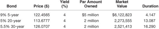
In this illustration it is assumed that the next coupon payment for each bond is exactly six months from now (i.e., there is no accrued interest). The market value for the portfolio is $10,917,791. Since each bond is option free, the modified duration can be used. The market price per $100 par value of each bond, its yield, and its duration are given below:

In this illustration, K is equal to 3 and:

w₁ = $6,122,823/$10,917,791 = 0.561 D₁ = 4.147

w₂ = $2,273,555/$10,917,791 = 0.208 D₂ = 13.087

w₃ = $2,521,413/$10,917,791 = 0.231 D₃ = 16.290

The portfolio’s duration is:

0.561 (4.147) + 0.208 (13.087) + 0.231 (16.290) = 8.81

A portfolio duration of 8.81 means that for a 100 basis point change in the yield of all three bonds, the market value of the portfolio will change by approximately 8.81%. But keep in mind that the yield on all three bonds must change by 100 basis points for the duration measure to be useful. This is a critical assumption, and its importance cannot be overemphasized.⁶

An alternative procedure for calculating the duration of a portfolio is to calculate the dollar price change for a given number of basis points for each security in the portfolio and then add up all the price changes. Dividing the total of the price changes by the initial market value of the portfolio produces a percentage price change that can be adjusted to obtain the portfolio’s duration.

For example, consider the three-bond portfolio shown above. Suppose that we calculate the dollar price change for each bond in the portfolio based on its respective duration for a 50 basis point change in yield. We would then have

Thus a 50 basis point change in all rates changes the market value of the three-bond portfolio by $481,096. Since the market value of the portfolio is $10,917,791, a 50 basis point change produced a change in value of 4.41% ($481,096 divided by $10,917,791). Since duration is the approximate percentage change for a 100 basis point change in rates, this means that the portfolio duration is 8.82 (found by doubling 4.41). This is the same value for the portfolio’s duration as found earlier.

The spread duration for a portfolio or a bond index is computed as a market-weighted average of the spread duration for each sector.

Contribution to Portfolio Duration

Some portfolio managers look at exposure of a portfolio or a benchmark index to an issue or to a sector simply in terms of the market value percentage of that issue or sector in the portfolio. A better measure of exposure to an individual issue or sector is its contribution to portfolio duration or contribution to benchmark index duration. This is found by multiplying the percentage of the market value of the portfolio represented by the individual issue or sector by the duration of the individual issue or sector. That is,

Contribution to portfolio duration = weight of issue or sector in portfolio × duration of issue or sector

Contribution to benchmark index duration = weight of issue or sector in benchmark index × duration of issue or sector

A portfolio manager who wants to determine the contribution of a sector to portfolio duration relative to the contribution of the same sector in a broad-based market index can compute the difference between the two contributions. The difference in the percentage distribution by sector is not as meaningful as is the difference in the contribution to duration.

CONVEXITY

The duration measure indicates that regardless of whether interest rates increase or decrease, the approximate percentage price change is the same. However, as we noted earlier, this is not consistent with Property 3 of a bond’s price volatility. Specifically, while for small changes in yield the percentage price change will be the same for an increase or decrease in yield, for large changes in yield this is not true. This suggests that duration is only a good approximation of the percentage price change for small changes in yield.

We demonstrated this property earlier using a 5% 20-year bond selling to yield 4% with a duration of 13.09. For a 10 basis point change in yield, the estimate was accurate for both an increase or a decrease in yield. However, for a 200 basis point change in yield, the approximate percentage price change was off considerably.

The reason for this result is that duration is in fact a first (linear) approximation for a small change in yield.⁷ The approximation can be improved by using a second approximation. This approximation is referred to as “convexity.” The use of this term in the industry is unfortunate because the term convexity is also used to describe the shape or curvature of the price/yield relationship. The convexity measure of a security can be used to approximate the change in price that is not explained by duration.

Convexity Measure

The convexity measure of a bond is approximated using the following formula:

where the notation is the same as used earlier for duration as given by Eq. (7–1).

For our hypothetical 5% 20-year bond selling to yield 4%, we know that for a 20 basis point change in yield (y = 0.002),

V₀ = 113.6777, V₋ = 116.7049, and V₊ = 110.7527

Substituting these values into the convexity measure given by Eq. (7–4) gives

We’ll see how to use this convexity measure shortly. Before doing so, there are three points that should be noted. First, there is no simple interpretation of the convexity measure. Second, in contrast to duration, it is more common for market participants to refer to the value computed in Eq. (7–4) as the “convexity of a bond” rather than the “convexity measure of a bond.” Finally, the convexity measure reported by dealers and vendors will differ for an option-free bond. The reason is that the value obtained from Eq. (7–4) is often scaled for the reason explained after we demonstrate how to use the convexity measure.

Convexity Adjustment to Percentage Price Change

Given the convexity measure, the approximate percentage price change adjustment due to the bond’s convexity (i.e., the percentage price change not explained by duration) is

For example, for the 5% coupon bond maturing in 20 years, the convexity adjustment to the percentage price change based on duration if the yield increases from 4% to 6% is

112.38 × (0.02)² × 100 = 4.50%

If the yield decreases from 4% to 2%, the convexity adjustment to the approximate percentage price change based on duration also would be 4.50%.

The approximate percentage price change based on duration and the convexity adjustment is found by adding the two estimates. Thus, for example, if yields change from 4% to 6%, the estimated percentage price change would be

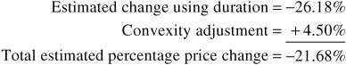
The actual percentage price change is –22.20%.

For a decrease of 200 basis points, from 4% to 2%, the approximate percentage price change would be as follows:

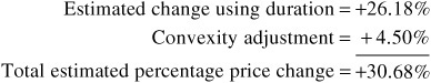
The actual percentage price change is +31.29%. Thus duration combined with the convexity adjustment does a better job of estimating the sensitivity of a bond’s price change to large changes in yield.

Notice that when the convexity measure is positive, we have the situation described earlier that the gain is greater than the loss for a given large change in rates. That is, the bond exhibits positive convexity. We can see this in the preceding example. However, if the convexity measure is negative, we have the situation where the loss will be greater than the gain. For example, suppose that a callable bond has an effective duration of 4 and a convexity measure of –30. This means that the approximate percentage price change for a 200 basis point change is 8%. The convexity adjustment for a 200 basis point change in rates is then

–30 × (0.02)² × 100 = –1.2

The convexity adjustment is –1.2%, and therefore, the bond exhibits the negative convexity property illustrated in Exhibit 7–7. The approximate percentage price change after adjusting for convexity is

For a decrease of 200 basis points, the approximate percentage price change would be as follows:

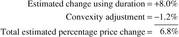
Notice that the loss is greater than the gain—a property called negative convexity that we discussed earlier and illustrated in Exhibit 7–7.

Scaling the Convexity Measure

The convexity measure as given by Eq. (7–4) means nothing in isolation. It is the substitution of the computed convexity measure into Eq. (7–5) that provides the estimated adjustment for convexity. Therefore, it is possible to scale the convexity measure in any way and obtain the same convexity adjustment.

For example, in some books the convexity measure is defined as follows:

Equation (7–6) differs from Eq. (7–4) because it does not include 2 in the denominator. Thus the convexity measure computed using Eq. (7–6) will be double the convexity measure using Eq. (7–4). Thus, for our earlier illustration, since the convexity measure using Eq. (7–4) is 112.38, the convexity measure using Eq. (7–6) would be 224.76.

Which is correct, 112.38 or 224.76? The answer is both. The reason is that the corresponding equation for computing the convexity adjustment would not be given by Eq. (7–5) if the convexity measure is obtained from Eq. (7–6). Instead, the corresponding convexity adjustment formula would be

Equation (7–7) differs from Eq. (7–5) in that the convexity measure is divided by 2. Thus the convexity adjustment will be the same whether one uses Eq. (7–4) to get the convexity measure and Eq. (7–5) to get the convexity adjustment or one uses Eq. (7–6) to compute the convexity measure and Eq. (7–7) to determine the convexity adjustment.

Some dealers and vendors scale the convexity measure in a different way. One also can compute the convexity measure as follows:

Equation (7–8) differs from Eq. (7–4) by the inclusion of 100 in the denominator. In our illustration, the convexity measure would be 1.1238 rather than 112.38 using Eq. (7–4). The convexity adjustment formula corresponding to the convexity measure given by Eq. (7–8) is then

Similarly, one can express the convexity measure as shown in Eq. (7–10):

For the bond we have been using in our illustrations, the convexity measure is 2.2476. The corresponding convexity adjustment is

Consequently, the convexity measures (or just simply “convexity” as it is referred to by some market participants) that could be reported for this option-free bond are 112.38, 224.76, 1.1238, and 2.2476. All these values are correct, but they mean nothing in isolation. To use them to obtain the convexity adjustment to the price change estimated by duration requires knowing how they are computed so that the correct convexity adjustment formula is used. It is the convexity adjustment that is important—not the convexity measure in isolation.

It is also important to understand this when comparing the convexity measures reported by dealers and vendors. For example, if one dealer shows a portfolio manager bond A with a duration of 4 and a convexity measure of 50, and a second dealer shows the manager bond B with a duration of 4 and a convexity measure of 80, which bond has the greater percentage price change response to changes in interest rates? Since the duration of the two bonds is identical, the bond with the larger convexity measure will change more when rates decline. However, not knowing how the two dealers computed the convexity measure means that the manager does not know which bond will have the greater convexity adjustment. If the first dealer used Eq. (7–4) and the second dealer used Eq. (7–6), then the convexity measures must be adjusted in terms of either equation. For example, using Eq. (7–4), the convexity measure of 80 computed using Eq. (7–6) is equal to a convexity measure of 40 based on Eq. (7–4).

Modified Convexity and Effective Convexity

The prices used in Eq. (7–4) to calculate convexity can be obtained by assuming that when the yield changes the expected cash-flows either do not change or they do change. In the former case, the resulting convexity is called modified convexity. (Actually, in the industry, convexity is not qualified by the adjective modified.) In contrast, effective convexity assumes that the cash-flows do change when yields change. This is the same distinction made for duration.

As with duration, there is little difference between modified convexity and effective convexity for option-free bonds. However, for bonds with embedded options, there can be quite a difference between the calculated modified convexity and the effective convexity measures. In fact, for all option-free bonds, either convexity measure will have a positive value. For bonds with embedded options, the calculated effective convexity can be negative when the calculated modified convexity measure is positive.

Illustrations of Effective Duration and Convexity

As noted earlier, modified duration and effective duration are two ways to measure the price sensitivity of a fixed income security. Modified duration ignores any effect on cash-flows that might take place as a result of changes in interest rates. Effective duration does not ignore the potential for such changes in cash-flows. For example, bonds with embedded options will have very different cash-flow properties as interest rates (or yields) change. Modified duration ignores these effects completely. In order to apply effective duration, an available interest-rate model and corresponding valuation model are needed. The example in this section shows how to compute the effective duration of securities with cash-flows that are dependent on interest rates.

There is no difference between modified and effective duration for option-free or straight bonds. In fact, it can be shown that they are mathematically identical when the change in rates (or yields) becomes very small. As shown in the example, even for bonds with embedded options, the differences between the two measures are minimal over certain ranges of yields. For example, when the embedded option is far out-of-the-money, the cash-flows of the bond are not affected by small changes in yields, resulting in almost no difference in cash-flows between the two measures.

Convexity (sometimes referred to as “standard convexity”) suffers the same limitations as modified duration and therefore is not generally useful for securities with embedded options. However, similar to the duration measures, in ranges of rates (or yields) where the cash-flows are not materially affected by small changes in yields, the two convexity measures are almost identical.

The following example illustrates how to calculate and interpret effective duration and effective convexity for option-free bonds and bonds with embedded options.

Suppose that we need to measure the interest-rate sensitivity of the following three securities:

1. A five-year 2.50% coupon option-free semiannual coupon bond with a current price of 97.69% of par

2. A five-year 2.25% coupon bond, callable at par in years 2 through 5 on the semiannual coupon dates, with a current price of 96.54% of par

3. A five-year 2.75% coupon bond, putable at par in years 2 through 5 on the semiannual coupon dates, with a current price of 100.4410453 of par

The cash-flows of these securities are very different as interest rates change. Consequently, the sensitivities to changes in interest rates are also very different.

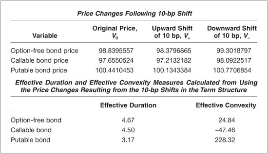
Using an interest-rate model that is based on the existing term structure,⁸ the term structure of interest rates is shifted up and down by 10 basis points (bps), and the resulting price changes are recorded. Using the notation for duration and convexity earlier in this chapter, V₋ corresponds to the price after a downward shift in interest rates, V₊ corresponds to the price after an upward shift in interest rates, V₀ is the current price, and y is the assumed shift in the term structure.⁹ Exhibit 7–15 shows these prices for each bond using Eq. (7–1) for duration and Eq. (7–6) for the convexity measure.

It is very important to realize the importance of the valuation model in this exercise. The model must account for the change in cash-flows of the securities as interest rates change. The callable and putable bonds have very different cash-flow characteristics that depend on the level of interest rates. The valuation model used must account for this property. (Note that when calculating the measures, users are cautioned not to round values. Since the denominators of both the duration and convexity terms are very small, any rounding will have a significant impact on results.)

Option-Free Bond

The effective duration for the straight bond is found by recording the price changes from shifting the term structure up (V₊) and down (V₋) by 10 bps and then substituting these values into Eq. (7–1). The prices are shown in Exhibit 7–15. Consequently, the computation is

EXHIBIT 7–15
Original Prices and Resulting Prices from a Downward and Upward 10 Basis Point Interest-Rate Shift and the Corresponding Effective Duration and Effective Convexity for Three Bonds Based on the Black-Derman-Toy Model

Similarly, the calculation for effective convexity is found by substituting the corresponding prices into Eq. (7–6):

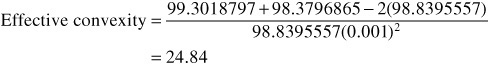
For the option-free bond, the modified duration is 4.67 and the convexity is 24.84. These are very close to the effective measures shown in Exhibit 7–15. This demonstrates that, for option-free bonds, the two measures are almost the same for small changes in yields.

Exhibit 7–16 shows the effects of the term structure shifts on the effective duration and effective convexity of the option-free bond. The effective duration increases as yields decrease because as yields decrease the slope of the price/yield relationship for option-free bonds becomes steeper and effective duration (and modified duration) is directly proportional to the slope of this relationship. For example, the effective duration at very low yields (−250-bp shift) is 4.74 and decreases to 4.44 at very high rates (+1,000 bps). Exhibit 7–17 illustrates this phenomenon; as yields increase, notice how the slope of the price/yield relationship decreases (becomes more horizontal or flatter).

EXHIBIT 7–16
Effective Duration and Effective Convexity for Various Shifts in the Term Structure for Three Bonds

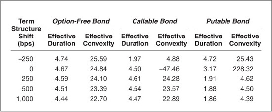
EXHIBIT 7–17
Price/Yield Relationship of the Option-Free Bond

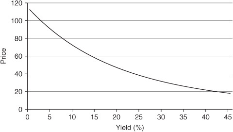
As the term structure shifts up (i.e., as rates rise), the yield to maturity on an option-free bond increases by approximately the same amount. As the yield increases, the bond’s convexity decreases. Exhibit 7–17 illustrates this property. As yields increase, the curvature (or the rate of change of the slope) decreases. The results in Exhibit 7–16 for the option-free bond also bear this out. The effective convexity values become smaller as yields increase. For example, the effective convexity at very low yields (−250-bp shift) is 25.59 and decreases to 22.70 at very high rates (+1,000-bp shift).

These are both well-documented properties of option-free bonds. The modified duration and convexity numbers for the option-free bond are almost identical to the effective measures for the option-free bond shown in Exhibit 7–16.

Callable Bond

The effective duration for the callable bond is found by recording the price changes from shifting the term structure up (V₊) and down (V₋) by 10 bps and then substituting these values into Eq. (7–1). The prices are shown in Exhibit 7–15. Note that these prices take into account the changing cash-flows resulting from the embedded call option. Consequently, the computation is

Similarly, the calculation for effective convexity is found by substituting the corresponding prices into Eq. (7–6):

The relationship between the shift in rates and effective duration is shown in Exhibit 7–16 and in Exhibit 7–18. As rates increase, the effective duration of the callable bond becomes larger. For example, the effective duration at very low yields (−250-bp shift) is 1.97 and increases to 4.47 at very high rates (+1,000 bps). This reflects the fact that as rates increase, the likelihood of the bond being called decreases, and as a result, the bond behaves more like an option-free bond; hence its effective duration increases. Conversely, as rates drop, this likelihood increases, and the bond and its effective duration behave more like a bond with a two-year maturity because of the call option becoming effective in two years. As rates decrease significantly, the likelihood of the issuer calling the bond in two years increases. Consequently, at very low and intermediate rates, the difference between the effective duration measure and modified duration is large, and at very high rates, the difference is small.

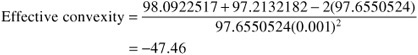
EXHIBIT 7–18
Price /Yield Relationship of the Callable Bond

Effective convexity measures the curvature of the price/yield relationship of bonds. Low values for effective convexity simply mean that the relationship is becoming linear (an effective convexity of zero represents a linear relationship). As shown in Exhibit 7–16, the effective convexity values of the callable bond at extremely low interest rates (i.e., for the −250-bp shift in the term structure) are very small positive numbers 4.88. This means that the relationship is almost linear but exhibits slight convexity. This is due to the call option being delayed by two years. At these extremely low interest rates, the callable bond exhibits slight positive convexity because the price compression at the call price is not complete for another two years.¹⁰ If this bond were immediately callable, the price/yield relationship would exhibit positive convexity at high-yields and negative convexity at low yields. At the current level of interest rates, the effective convexity is negative, as expected. At these rate levels, the embedded call option causes enough price compression to cause the curvature of the price/yield relationship to be negatively convex (i.e., concave). Exhibit 7–18 illustrates these properties. It is at these levels that the embedded option has a significant effect on the cash-flows of the callable bond.

Exhibit 7–16 shows that for large positive yield-curve shifts (i.e., for the +250-bp, +500-bp, and +1,000-bp shifts in the term structure), the effective convexity of the callable bond becomes positive and very close to the effective convexity values of the straight bond. For example, the effective convexity at the +250-bp shift is 24.28 for the callable bond and 24.10 for the straight bond. The only reason they are not the same is because the coupon rates of the bonds are not equal. Consequently, at very low and intermediate rates, the difference between effective convexity and standard convexity is large, and at very high rates, the difference is small. The intuition behind these findings is straightforward. At low rates, the cash-flows of the callable bond are severely affected by the likelihood of the embedded call option being exercised by the issuer. At high rates, the embedded call option is so far out-of-the-money that it has almost no effect on the cash-flows of the callable bond, and so the callable bond behaves like an option-free bond.

Putable Bond

The effective duration for the putable bond is found by recording the price changes from shifting the term structure up (V₊) and down (V₋) by 10 bps and then substituting these values into Eq. (7–1). The prices are shown in Exhibit 7–15. Note that these prices take into account the changing cash-flows resulting from the embedded put option. Consequently, the computation is

Similarly, the calculation for effective convexity is found by substituting the corresponding prices into Eq. (7–6):

Because the putable bond behaves so differently from the other two bonds, the effective duration and effective convexity values are very different. As rates increase, the bond behaves more like a two-year bond because the owner will, in all likelihood, exercise his right to put the bond back at the put price as soon as possible. As a result, the effective duration of the putable bond is expected to decrease as rates increase. This is due to the embedded put option severely affecting the cash-flows of the putable bond. Conversely, as rates fall, the putable bond behaves more like a five-year straight bond because the embedded put option is so far out-of-the-money and has little effect on the cash-flows of the putable bond. Effective duration should reflect these properties. Exhibit 7–16 shows that this is indeed the case. For example, the effective duration at very low yields (−250-bp shift) is 4.72 and decreases to 1.86 at very high rates (+1,000 bps). Consequently, at very high and intermediate rates, the difference between the effective duration and modified duration measures is large, and at low rates, the difference is small.

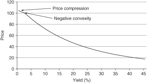
Exhibit 7–16 shows that the effective convexity of the putable bond is positive for all rate shifts, as would be expected, but it becomes smaller as rates increase (i.e., for the +250-bp, +500-bp, and +1,000-bp shifts in the term structure). As rates increase, the putable bond price/yield relationship will become linear because of the bond’s price truncation at the put price.¹¹ This is the reason for the small effective convexity values for the putable bond for the three positive shifts in the term structure (4.62, 4.50, and 4.39, respectively). It is at these levels that the embedded put option has a significant effect on the cash-flows of the putable bond. Consequently, at very high and intermediate rates, the difference between the effective convexity and standard convexity is very large. Exhibit 7–19 illustrates these properties.

EXHIBIT 7–19
Price/Yield Relationship of the Putable Bond

At very low rates (i.e., for the 250-bp downward shift in the term structure), the putable bond behaves like a five-year straight bond because the put option is so far out-of-the-money. Therefore, as the term structure is shifted downward, the putable bond’s effective convexity values approach those of a comparable five-year option-free bond. Comparing the effective convexity measures for the putable bond and the option-free bond illustrates this characteristic. For example, the effective convexity at the −250-bp shift is 25.43 for the putable bond and 25.59 for the option-free bond. The two convexity measures are almost identical. In fact, they would be identical if their coupon rates were equal.

Exhibit 7–19 illustrates these properties. Also notice how the transition from low yields to high-yields forces the price/yield relationship to have a very high convexity at intermediate levels of yields. For example, the current effective convexity of the putable bond is 228.32 compared with 24.84 for the straight bond and 47.46 for the callable bond. This is so because as yields increase, the embedded put option moves from out-of-the-money to in, and the behavior of the bond goes from that of a five-year bond to a two-year bond as a result. This corresponding price truncation causes the price/yield relationship to have to transition very quickly from the five-year (high effective duration) to the two-year (low effective duration), resulting in very high effective convexity.

Putting It All Together

Notice in Exhibit 7–16 how effective duration changes much more across yields for the callable and putable bonds than it does for the option-free bond. This is to be expected because the embedded options have such a significant influence over cash-flows as yields change over a wide spectrum. Interestingly, at high (low) yields, the callable (putable) bond’s effective duration is very close to the option-free bond. This is where the embedded call (put) option is so far out-of-the-money that the two securities behave similarly. The same intuition holds for the effective convexity measures.

As explained and illustrated earlier, the common use of effective duration and effective convexity is to estimate the percentage price changes in fixed income securities for assumed changes in yield. In fact, it is not uncommon for effective duration and effective convexity to be presented in terms of estimated percentage price change for a given change in yield (typically 100 bp). Exhibits 7–20 and 7–21 show this alternative presentation for a ±100-bp change in yield using Eqs. (7–2) and (7–7).

EXHIBIT 7–20
Using Effective Duration and Effective Convexity to Illustrate the impact of 100 bps Increase in Yield Across Different Term Structure Levels

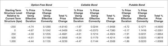
EXHIBIT 7–21
Using Effective Duration and Effective Convexity to Illustrate the Impact of 100 bps Decline in Yield Across Different Term Structure Levels

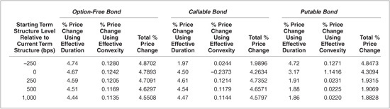
PRICE VALUE OF A BASIS POINT

Some managers use another measure of the price volatility of a bond to quantify interest-rate risk—the price value of a basis point (PVBP). This measure, also called the dollar value of an 01 (DV01), is the absolute value of the change in the price of a bond for a 1 basis point change in yield. That is,

PVBP = | initial price – price if yield is changed by 1 basis point |

Does it make a difference if the yield is increased or decreased by 1 basis point? It does not because of Property 2—the change will be about the same for a small change in basis points.

To illustrate the computation, we use the values in Exhibit 7–4. If the initial yield is 4%, we can compute the PVBP by using the prices for either the yield at 3.99% or 4.01%. The PVPB for both for each bond is shown below:

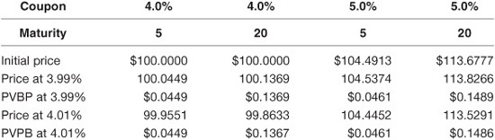
The PVBP is related to duration. In fact, PVBP is simply a special case of dollar duration. We know that the duration of a bond is the approximate percentage price change for a 100 basis point change in interest rates. We also know how to compute the approximate percentage price change for any number of basis points given a bond’s duration using Eq. (7–2). Given the initial price and the approximate percentage price change for 1 basis point, we can compute the change in price for a 1 basis point change in rates.

For example, consider the 5% 20-year bond. The duration for this bond is 13.09. Using Eq. (7–2), the approximate percentage price change for a 1 basis point increase in interest rates (i.e., y = 0.0001) ignoring the negative sign in Eq. (7–2) is

13.09 × (0.0001) × 100 = 0.1309%

Given the initial price of 113.6777, the dollar price change estimated using duration is

0.1309% × 113.6777 = $0.1488

This is the same price change as shown above for a PVPB for this bond. Below is (1) the PVPB based on a 1 basis point increase for each bond and (2) the estimated price change using duration for a 1 basis point increase for each bond:

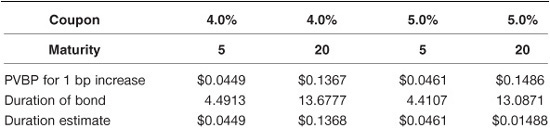
THE IMPORTANCE OF YIELD VOLATILITY

What we have not considered thus far is the volatility of interest rates. All other factors equal, the higher the coupon rate, the lower is the price volatility of a bond to changes in interest rates. In addition, the higher the level of yields, the lower is the price volatility of a bond to changes in interest rates. This is illustrated in Exhibit 7–22, which shows the price/yield relationship for an option-free bond. When the yield level is high (Y_H in the exhibit), a change in interest rates does not produce a large change in the initial price (P_H in the exhibit). However, when the yield level is low (Y_L in the exhibit), a change in interest rates of the same number of basis points as shown when the yield is high does produce a large change in the initial price (P_L in the exhibit).

EXHIBIT 7–22
The Effect of Yield Level on Price Volatility

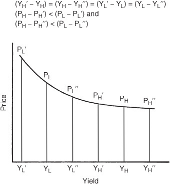
This also can be cast in terms of duration properties: the higher the coupon, the lower is the duration, and the higher the yield level, the lower is the duration. Given these two properties, a 10-year non-investment-grade bond has a lower duration than a current coupon 10-year Treasury note because the former has a higher coupon rate and trades at a higher yield level. Does this mean that a 10-year non-investment-grade bond has less interest-rate risk than a current coupon 10-year Treasury note? Consider also that a 10-year Swiss government bond has a lower coupon rate than a current coupon 10-year U.S. Treasury note and trades at a lower yield level. Therefore, a 10-year Swiss government bond will have a higher duration than a current coupon 10-year Treasury note. Does this mean that a 10-year Swiss government bond has greater interest-rate risk than a current coupon 10-year U.S. Treasury note? The missing link is the relative volatility of rates, which we shall call yield volatility or interest-rate volatility.

The greater the expected yield volatility, the greater is the interest-rate risk for a given duration and current value of a position. In the case of non-investment-grade bonds, while their durations are less than current coupon Treasuries of the same maturity, the yield volatility of non-investment-grade bonds is greater than that of current coupon Treasuries. For the 10-year Swiss government bond, while the duration is greater than for a current coupon 10-year U.S. Treasury note, the yield volatility of 10-year Swiss bonds is considerably less than that of 10-year U.S. Treasury notes.

A framework that ties together the price sensitivity of a bond position to rate changes and yield volatility is the value-at-risk (VaR) framework. Risk in this framework is defined as the maximum estimated loss in market value of a given position that is expected to happen with a specified probability.

KEY POINTS

• The full-valuation approach to interest-rate risk management involves repricing bonds under different interest rate scenarios to quantify price sensitivity to interest-rate changes.

• Important bond price volatility properties for option-free bonds are (1) prices move inversely to yields, but percentage price changes are not the same for all bonds; (2) for small changes in yield, the percentage price change is roughly the same, whether yields increase or decrease; (3) for large changes in yield, the percentage price change is not the same for yield increases compared with yield decreases, and; (4) for a given large change in yield, the percentage price increase is greater than the percentage price decrease.

• Bond features affect interest-rate risk. For option-free bonds, a longer maturity leads to more interest-rate risk, a higher coupon rate leads to less interest-rate risk, and interest-rate risk is greater at lower yields. Additionally, embedded options affect interest-rate risk.

• An alternative to the full-valuation approach is the duration/convexity approach. Duration is the approximate percentage price change in a bond’s value for a 100 basis point change in rates.

• Duration assumes the term structure is flat and all interest-rate changes result from parallel shifts.

• Convexity adjustments improve duration estimates, particularly for large interest-rate changes.

• Bonds with embedded options, such as the issuer’s right to call the bond or an investor’s right to put the bond, have cash-flows that change as interest rates change. Effective duration accounts for changes in the bond’s cash-flow. For this purpose, a term structure model is required.

• Callable bonds exhibit negative convexity and price compression at low interest rates. Putable bonds exhibit price truncation at high-yields and high convexity at low yields.