
CHAPTER
EIGHT
THE STRUCTURE OF INTEREST RATES
FRANK J. FABOZZI, PH.D., CFA, CPA
Professor of Finance
EDHEC Business School
There is no single interest rate for any economy; rather, there is an interdependent structure of interest rates. The interest rate that a borrower has to pay depends on a myriad of factors. In this chapter we describe these factors. We begin with a discussion of the base interest rate: the interest rate on U.S. government securities. Next, we explain the factors that affect the yield spread or risk premium for non-Treasury securities. Finally, we focus on one particular factor that affects the interest rate demanded in an economy for a particular security: maturity. The relationship between yield and maturity (or term) is called the term structure of interest rates, and this relationship is critical in the valuation of securities. Determinants of the general level of interest rates in the economy will not be discussed.
THE BASE INTEREST RATE
The securities issued by the U.S. Department of the Treasury are backed by the full faith and credit of the U.S. government. Despite the credit concerns arising from the U.S. budget deficit and the downgrading of the U.S. government credit rating from triple A to AA+ by the credit rating agency of Standard & Poor’s in August 2011 (Moody’s and Fitch still maintained a triple A rating), market participants throughout the world view U.S. government obligations as having minimal credit risk. Therefore, interest rates on Treasury securities are the benchmark interest rates throughout the U.S. economy. The large sizes of Treasury issues have contributed to making the Treasury market the most active and hence the most liquid market in the world.
The minimum interest rate or base interest rate that investors will demand for investing in a non-Treasury security is the yield offered on a comparable maturity for an on-the-run Treasury security. The base interest rate is also referred to as the benchmark interest rate.
RISK PREMIUM
Market participants describe interest rates on non-Treasury securities as trading at a spread to a particular on-the-run Treasury security. For example, if the yield on a 10-year non-Treasury security is 5% and the yield on a 10-year Treasury security is 4%, the spread is 100 basis points. This spread reflects the additional risks the investor faces by acquiring a security that is not issued by the U.S. government and therefore can be called a risk premium. Thus we can express the interest rate offered on a non-Treasury security as
Base interest rate + spread
or equivalently,
Base interest rate + risk premium
The factors that affect the spread include (1) the type of issuer, (2) the issuer’s perceived creditworthiness, (3) the term or maturity of the instrument, (4) provisions that grant either the issuer or the investor the option to do something, (5) the taxability of the interest received by investors, and (6) the expected liquidity of the issue.
Types of Issuers
A key feature of a debt obligation is the nature of the issuer. In addition to the U.S. government, there are agencies of the U.S. government, municipal governments, corporations (domestic and foreign), and foreign governments that issue bonds.
The bond market is classified by the type of issuer. These are referred to as market sectors. The spread between the interest rate offered in two sectors of the bond market with the same maturity is referred to as an intermarket-sector spread.
Excluding the Treasury market sector, other market sectors have a wide range of issuers, each with different abilities to satisfy bond obligations. For example, within the corporate market sector, issuers are classified as utilities, transportations, industrials, and banks and finance companies. The spread between two issues within a market sector is called an intramarket-sector spread.
Perceived Creditworthiness of Issuer
Default risk or credit risk refers to the risk that the issuer of a bond may be unable to make timely payment of principal or interest payments. Most market participants rely primarily on commercial rating companies (Fitch Ratings, Moody’s Investors Service, and Standard & Poor’s) to assess the default risk of an issuer. The spread between Treasury securities and non-Treasury securities that are identical in all respects except for quality is referred to as a credit spread or quality spread.
Term-to-Maturity
As we explained in Chapter 6, the price of a bond will fluctuate over its life as yields in the market change. As demonstrated in Chapter 7, the volatility of a bond’s price is dependent on its maturity. With all other factors constant, the longer the maturity of a bond, the greater is the price volatility resulting from a change in market yields.
The spread between any two maturity sectors of the market is called a yield-curve spread or maturity spread. The relationship between the yields on comparable securities with different maturities, as mentioned earlier, is called the term structure of interest rates.
The term-to-maturity topic is very important, and we have devoted more time to this topic later in this chapter.
Inclusion of Options
It is not uncommon for a bond issue to include a provision that gives the bondholder or the issuer an option to take some action against the other party. An option that is included in a bond issue is referred to as an embedded option. We discussed the various types of embedded options in Chapter 1. The most common type of option in a bond issue is the call provision, which grants the issuer the right to retire the debt, fully or partially, before the scheduled maturity date. The inclusion of a call feature benefits issuers by allowing them to replace an old bond issue with a lower-interest-cost issue when interest rates in the market decline. In effect, a call provision allows the issuer to alter the maturity of a bond. The exercise of a call provision is disadvantageous to the bondholder because the bondholder must reinvest the proceeds received at a lower interest rate.
The presence of an embedded option affects both the spread of an issue relative to a Treasury security and the spread relative to otherwise comparable issues that do not have an embedded option. In general, market participants will require a larger spread to a comparable Treasury security for an issue with an embedded option that is favorable to the issuer (such as a call option) than for an issue without such an option. In contrast, market participants will require a smaller spread to a comparable Treasury security for an issue with an embedded option that is favorable to the investor (such as a put option or a conversion option). In fact, the interest rate on a bond with an option that is favorable to an investor may be less than that on a comparable Treasury security.
Taxability of Interest
Unless exempted under the federal income tax code, interest income is taxable at the federal level. In addition to federal income taxes, there may be state and local taxes on interest income.
The federal tax code specifically exempts the interest income from qualified municipal bond issues. Because of this tax exemption, the yield on municipal bonds is less than on Treasuries with the same maturity. The difference in yield between tax-exempt securities and Treasury securities is typically measured not in basis points but in percentage terms. More specifically, it is measured as the percentage of the yield on a tax-exempt security relative to a comparable Treasury security.
The yield on a taxable bond issue after federal income taxes are paid is equal to
After-tax yield = pretax yield × (1 – marginal tax rate)
For example, suppose that a taxable bond issue offers a yield of 4% and is acquired by an investor facing a marginal tax rate of 35%. The after-tax yield would be
After-tax yield = 0.04 × (1 – 0.35) = 0.026 = 2.60%
Alternatively, we can determine the yield that must be offered on a taxable bond issue to give the same after-tax yield as a tax-exempt issue. This yield is called the equivalent taxable yield and is determined as follows:
![]()
For example, consider an investor facing a 35% marginal tax rate who purchases a tax-exempt issue with a yield of 2.6%. The equivalent taxable yield is then
![]()
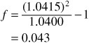
Notice that the lower the marginal tax rate, the lower is the equivalent taxable yield. For example, in our previous example, if the marginal tax rate is 25% rather than 35%, the equivalent taxable yield would be 3.47% rather than 4%, as shown below.
![]()
State and local governments may tax interest income on bond issues that are exempt from federal income taxes. Some municipalities exempt interest income from all municipal issues from taxation; others do not. Some states exempt interest income from bonds issued by municipalities within the state but tax the interest income from bonds issued by municipalities outside the state. The implication is that two municipal securities of the same quality rating and the same maturity may trade at some spread because of the relative demand for bonds of municipalities in different states. For example, in a high-income-tax state such as New York, the demand for bonds of municipalities will drive down their yield relative to municipalities in a low-income-tax state such as Florida, holding all credit issues aside.
Municipalities are not permitted to tax the interest income from securities issued by the U.S. Treasury. Thus part of the spread between Treasury securities and taxable non-Treasury securities of the same maturity reflects the value of the exemption from state and local taxes.
Expected Liquidity of an Issue
Bonds trade with different degrees of liquidity. The greater the expected liquidity at which an issue will trade, the lower is the yield that investors require. As noted earlier, Treasury securities are the most liquid securities in the world. The lower yield offered on Treasury securities relative to non-Treasury securities reflects the difference in liquidity as well as perceived credit risk. Even within the Treasury market, on-the-run issues have greater liquidity than off-the-run issues.
THE TERM STRUCTURE OF INTEREST RATES
In future chapters we will see the key role that the term structure of interest rates plays in the valuation of bonds. For this reason, we devote a good deal of space to this important topic.
The Yield Curve
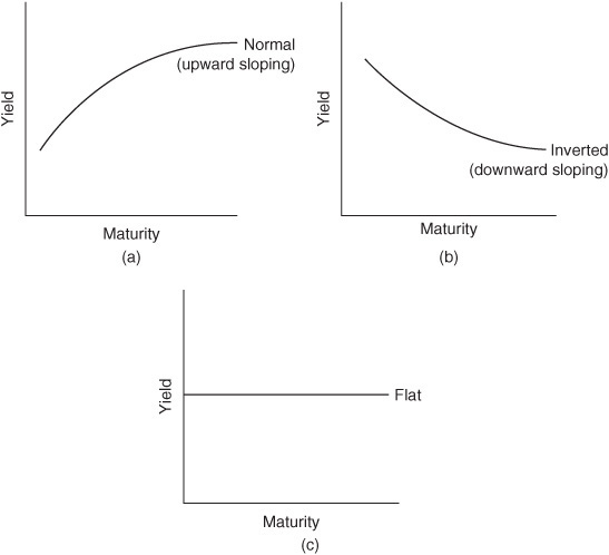
The graphic depiction of the relationship between the yield on bonds of the same credit quality but different maturities is known as the yield curve. In the past, most market participants have constructed yield curves from the observations of prices and yields in the Treasury market. Two reasons account for this tendency. First, Treasury securities are free of default risk, and differences in creditworthiness do not affect yield estimates. Second, as the most active bond market, the Treasury market offers the fewest problems of illiquidity or infrequent trading. Exhibit 8–1 shows the shape of three hypothetical Treasury yield curves that have been observed in the United States, as well as other countries.
EXHIBIT 8–1
Three Hypothetical Yield Curves
From a practical viewpoint, as we explained earlier in this chapter, the key function of the Treasury yield curve is to serve as a benchmark for pricing bonds and setting yields in other sectors of the debt market. However, market participants are coming to realize that the traditionally constructed Treasury yield curve is an unsatisfactory measure of the relation between required yield and maturity. The key reason is that securities with the same maturity actually may carry different yields. As we will explain, this phenomenon reflects the impact of differences in the bonds’ coupon rates. Hence it is necessary to develop more accurate and reliable estimates of the Treasury yield curve. We will show the problems posed by traditional approaches to the Treasury yield curve, and we will explain the proper approach to building a yield curve. The approach consists of identifying yields that apply to zero-coupon bonds and, therefore, eliminates the problem of nonuniqueness in the yield-maturity relationship.
Using the Yield Curve to Price a Bond
The price of a bond is the present value of its cash flows. However, in our discussion of the pricing of a bond in Chapter 6, we assumed that one interest rate should be used to discount all the bond’s cash flows. The appropriate interest rate is the yield on a Treasury security with the same maturity as the bond plus an appropriate risk premium or spread.
However, there is a problem with using the Treasury yield curve to determine the appropriate yield at which to discount the cash flow of a bond. To illustrate this problem, consider two hypothetical five-year Treasury bonds, A and B. The difference between these two Treasury bonds is the coupon rate, which is 12% for A and 3% for B. The cash flow for these two bonds per $100 of par value for the 10 six-month periods to maturity would be as follows:

Because of the different cash flow patterns, it is not appropriate to use the same interest rate to discount all cash flows. Instead, each cash flow should be discounted at a unique interest rate that is appropriate for the time period in which the cash flow will be received. But what should be the interest rate for each period?
The correct way to think about bonds A and B is not as bonds but as packages of cash flows. More specifically, they are packages of zero-coupon instruments. Thus the interest earned is the difference between the maturity value and the price paid. For example, bond A can be viewed as 10 zero-coupon instruments: One with a maturity value of $6 maturing six months from now, a second with a maturity value of $6 maturing one year from now, a third with a maturity value of $6 maturing 1.5 years from now, and so on. The final zero-coupon instrument matures 10 six-month periods from now and has a maturity value of $106. Likewise, bond B can be viewed as 10 zero-coupon instruments: One with a maturity value of $1.50 maturing six months from now, one with a maturity value of $1.50 maturing one year from now, one with a maturity value of $1.50 maturing 1.5 years from now, and so on. The final zero-coupon instrument matures 10 six-month periods from now and has a maturity value of $101.50. Obviously, in the case of each coupon bond, the value or price of the bond is equal to the total value of its component zero-coupon instruments.
In general, any bond can be viewed as a package of zero-coupon instruments. That is, each zero-coupon instrument in the package has a maturity equal to its coupon payment date or, in the case of the principal, the maturity date. The value of the bond should equal the value of all the component zero-coupon instruments. If this does not hold, a market participant may generate riskless profits by stripping the security and creating stripped securities.
To determine the value of each zero-coupon instrument, it is necessary to know the yield on a zero-coupon Treasury with that same maturity. This yield is called the spot rate, and the graphic depiction of the relationship between the spot rate and its maturity is called the spot-rate curve. Because there are no zero-coupon Treasury debt issues with a maturity greater than one year, it is not possible to construct such a curve solely from observations of Treasury yields. Rather, it is necessary to derive this curve from theoretical considerations as applied to the yields of actual Treasury securities. Such a curve is called a theoretical spot-rate curve.
Constructing the Theoretical Spot-Rate Curve
The theoretical spot-rate curve is constructed from the yield curve based on the observed yields of Treasury bills and Treasury coupon securities. The process of creating a theoretical spot-rate curve in this way is called bootstrapping.1
To explain this process, we use the data for the hypothetical price, annualized yield (yield-to-maturity), and maturity of the 20 Treasury securities shown in Exhibit 8–2.
EXHIBIT 8–2
Maturity and Yield-to-Maturity for 20 Hypothetical Treasury Securities

Throughout the analysis and illustrations to come, it is important to remember that the basic principle of bootstrapping is that the value of a Treasury coupon security should be equal to the value of the package of zero-coupon Treasury securities that duplicates the coupon bond’s cash flow.
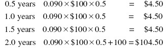
Consider the six-month Treasury bill in Exhibit 8–2. As explained in Chapter 9, a Treasury bill is a zero-coupon instrument. Therefore, its annualized yield of 8% is equal to the spot rate. Similarly, for the one-year Treasury bill, the cited yield of 8.3% is the one-year spot rate. Given these two spot rates, we can compute the spot rate for a theoretical 1.5-year zero-coupon Treasury. The price of a theoretical 1.5-year Treasury should equal the present value of three cash flows from an actual 1.5-year coupon Treasury, where the yield used for discounting is the spot rate corresponding to the cash flow. Using $100 as par, the cash flow for the 1.5-year coupon Treasury is as follows:

The present value of the cash flow is then
![]()
where
z1 = one-half the annualized six-month theoretical spot rate
z2 = one-half the one-year theoretical spot rate
z3 = one-half the 1.5-year theoretical spot rate
Because the six-month spot rate and one-year spot rate are 8.0% and 8.3%, respectively, we know that
z1 = 0.04 and z2 = 0.0415.
We can compute the present value of the 1.5-year coupon Treasury security as
![]()
Because the price of the 1.5-year coupon Treasury security (from Exhibit 8–2) is $99.45, the following relationship must hold:
![]()
We can solve for the theoretical 1.5-year spot rate as follows:
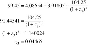
Doubling this yield, we obtain the bond-equivalent yield of 0.0893, or 8.93%, which is the theoretical 1.5-year spot rate. This rate is the rate that the market would apply to a 1.5-year zero-coupon Treasury security, if such a security existed.
Given the theoretical 1.5-year spot rate, we can obtain the theoretical two-year spot rate. The cash flow for the two-year coupon Treasury in Exhibit 8–2 is
The present value of the cash flow is then
![]()
where
z4 = one-half the two-year theoretical spot rate
Because the six-month spot rate, the one-year spot rate, and the 1.5-year spot rate are 8.0%, 8.3%, and 8.93%, respectively, then
z1 = 0.04 z2 = 0.0415 and z3 = 0.04465
Therefore, the present value of the two-year coupon Treasury security is
![]()
Because the price of the two-year coupon Treasury security is $99.64, the following relationship must hold:
![]()
We can solve for the theoretical two-year spot rate as follows:

Doubling this yield, we obtain the theoretical two-year spot rate bond-equivalent yield of 9.247%.
One can follow this approach sequentially to derive the theoretical 2.5-year spot rate from the calculated values of z1, z2, z3, and z4 (the six-month, one-year, 1.5-year, and two-year rates) and the price and coupon of the bond with a maturity of 2.5 years. Further, one could derive theoretical spot rates for the remaining 15 half-yearly rates. The spot rates thus obtained are shown in Exhibit 8–3. They represent the term structure of interest rates for maturities up to 10 years at the particular time to which the bond price quotations refer.
EXHIBIT 8–3
Theoretical Spot Rates

Why Treasuries Must Be Priced Based on Spot Rates
Financial theory tells us that the theoretical price of a Treasury security should be equal to the present value of the cash flows, where each cash flow is discounted at the appropriate theoretical spot rate. What we did not do, however, is demonstrate the economic force that ensures that the actual market price of a Treasury security does not depart significantly from its theoretical price.
To demonstrate this, we will use the 20 hypothetical Treasury securities introduced in Exhibit 8–2. The longest-maturity bond given in that exhibit is the 10-year, 12.5% coupon bond selling at par with a yield-to-maturity of 12.5%. Suppose that a government dealer buys the issue at par and strips it, expecting to sell the zero-coupon Treasury securities at the yields-to-maturity indicated in Exhibit 8–3 for the corresponding maturity.
Exhibit 8–4 shows the price that would be received for each zero-coupon Treasury security created. The price for each is the present value of the cash flow from the stripped Treasury discounted at the yield-to-maturity corresponding to the maturity of the security (from Exhibit 8–2). The total proceeds received from selling the zero-coupon Treasury securities created would be $104.1880 per $100 of par value of the original Treasury issue. This would result in an arbitrage profit of $4.1880 per $100 of the 10-year, 12.5% coupon Treasury security purchased.
EXHIBIT 8–4
Illustration of Arbitrage Profit from Coupon Stripping

To understand why the government dealer has the opportunity to realize this profit, look at the third column of Exhibit 8–4, which shows how much the government dealer paid for each cash flow by buying the entire package of cash flows (i.e., by buying the bond). For example, consider the $6.25 coupon payment in four years. By buying the 10-year Treasury bond priced to yield 12.5%, the dealer effectively pays a price based on 12.5% (6.25% semiannually) for that coupon payment or, equivalently, $3.8481. Under the assumptions of this illustration, however, investors were willing to accept a lower yield-to-maturity, 10.4% (5.2% semiannually), to purchase a zero-coupon Treasury security with four years to maturity. Thus investors were willing to pay $4.1663. On this one coupon payment, the government dealer realizes a profit equal to the difference between $4.1663 and $3.8481 (or $0.3182). From all the cash flows, the total profit is $4.1880. In this instance, coupon stripping shows that the sum of the parts is greater than the whole.
Suppose that instead of the observed yield-to-maturity from Exhibit 8–2, the yields investors want are the same as the theoretical spot rates shown in Exhibit 8–3. If we use these spot rates to discount the cash flows, the total proceeds from the sale of the zero-coupon Treasury securities would be equal to $100, making coupon stripping uneconomic.
In our illustration of coupon stripping, the price of the Treasury security is less than its theoretical price. Suppose instead that the price of the Treasury security is greater than its theoretical price. In such cases, investors can purchase a package of zero-coupon Treasury securities such that the cash flow of the package of securities replicates the cash flow of the mispriced coupon Treasury security. By doing so, the investor will realize a yield higher than the yield on the coupon Treasury security. For example, suppose that the market price of the 10-year Treasury security we used in our illustration (Exhibit 8–4) is $106. By buying the 20 zero-coupon bonds shown in Exhibit 8–4 with a maturity value identical to the cash flow shown in the second column, the investor is effectively purchasing a 10-year Treasury coupon security at a cost of $104.1880 instead of $106.
The process of coupon stripping and reconstituting prevents the actual spot-rate curve observed on zero-coupon Treasuries from departing significantly from the theoretical spot-rate curve. As more stripping and reconstituting occurs, forces of demand and supply will cause rates to return to their theoretical spot-rate levels. This is what has happened in the Treasury market.
Forward Rates
Consider an investor who has a one-year investment horizon and is faced with the following two alternatives:
Alternative 1: Buy a one-year Treasury bill.
Alternative 2: Buy a six-month Treasury bill, and when it matures in six months, buy another six-month Treasury bill.
The investor will be indifferent between the two alternatives if they produce the same return over the one-year investment horizon. The investor knows the spot rate on the six-month Treasury bill and the one-year Treasury bill. However, she does not know what yield will be available on a six-month Treasury bill that will be purchased six months from now. The yield on a six-month Treasury bill six months from now is called a forward rate. Given the spot rates for the six-month Treasury bill and the one-year bill, we wish to determine the forward rate on a six-month Treasury bill that will make the investor indifferent between the two alternatives. That rate can be readily determined.
At this point, however, we need to digress briefly and recall several present-value and investment relationships. First, if you invested in a one-year Treasury bill, you would receive $100 at the end of one year. The price of the one-year Treasury bill would be
![]()
where z2 is one-half the bond-equivalent yield of the theoretical one-year spot rate.
Second, suppose that you purchased a six-month Treasury bill for $X. At the end of six months, the value of this investment would be
X(1 + z1)
where z1 is one-half the bond-equivalent yield of the theoretical six-month spot rate.
Let f represent one-half the forward rate (expressed as a bond-equivalent basis) on a six-month Treasury bill available six months from now. If the investor were to renew her investment by purchasing that bill at that time, then the future dollars available at the end of one year from the $X investment would be
X(1 + z1)(1 + f)
Third, it is easy to use this formula to find out how many $X the investor must invest in order to get $100 one year from now. This can be found as follows:
X(1 + z1)(1 + f) = 100
which gives us
![]()
We are now prepared to return to the investor’s choices and analyze what that situation says about forward rates. The investor will be indifferent between the two alternatives confronting her if she makes the same dollar investment and receives $100 from both alternatives at the end of one year. That is, the investor will be indifferent if
![]()
Solving for f, we get
![]()
Doubling f gives the bond-equivalent yield for the six-month forward rate six months from now.
We can illustrate the use of this formula with the theoretical spot rates shown in Exhibit 8–3. From that exhibit, we know that
Six-month bill spot rate = 0.080 so z1 = 0.0400
One-year bill spot rate = 0.083 so z2 = 0.0415
Substituting into the formula, we have
Therefore, the forward rate on a six-month Treasury security, quoted on a bond-equivalent basis, is 8.6% (0.043 × 2). Let’s confirm our results. The price of a one-year Treasury bill with a $100 maturity value is
![]()
If $92.19 is invested for six months at the six-month spot rate of 8%, the amount at the end of six months would be
92.19(1.0400) = 95.8776
If $95.8776 is reinvested for another six months in a six-month Treasury offering 4.3% for six months (8.6% annually), the amount at the end of one year would be
95.8776(1.043) = 100
Both alternatives will have the same $100 payoff if the six-month Treasury bill yield six months from now is 4.3% (8.6% on a bond-equivalent basis). This means that if an investor is guaranteed a 4.3% yield (8.6% bond-equivalent basis) on a six-month Treasury bill six months from now, she will be indifferent between the two alternatives.
We used the theoretical spot rates to compute the forward rate. The resulting forward rate is also called the implied forward rate.
We can take this sort of analysis much further. It is not necessary to limit ourselves to implied forward rates six months from now. The yield curve can be used to calculate the implied forward rate for any time in the future for any investment horizon. For example, the following can be calculated:
• The two-year implied forward rate five years from now
• The six-year implied forward rate two years from now
• The seven-year implied forward rate three years from now
Relationship between Spot Rates and Short-Term Forward Rates
Suppose that an investor purchases a five-year zero-coupon Treasury security for $58.42 with a maturity value of $100. He could instead buy a six-month Treasury bill and reinvest the proceeds every six months for five years. The number of dollars that will be realized depends on the six-month forward rates. Suppose that the investor actually can reinvest the proceeds maturing every six months at the implied six-month forward rates. Let’s see how many dollars would accumulate at the end of five years. The implied six-month forward rates were calculated for the yield curve given in Exhibit 8–3. Letting ft denote the six-month forward rate beginning t six-month periods from now, the semiannual implied forward rates using the spot rates shown in that exhibit are as follows:

If he invests the $58.48 at the six-month spot rate of 4% (8% on a bond-equivalent basis) and reinvests at the forward rates shown above, the number of dollars accumulated at the end of five years would be
$58.48(1.04)(1.043)(1.05098)(1.051005)(1.05177)(1.056945) × (1.060965)(1.069310)(1.064625)(1.06283) = $100
Therefore, we see that if the implied forward rates are realized, the $58.48 investment will produce the same number of dollars as an investment in a five-year zero-coupon Treasury security at the five-year spot rate. From this illustration, we can see that the five-year spot rate is related to the current six-month spot rate and the implied six-month forward rates.
In general, the relationship between a t-period spot rate, the current six-month spot rate, and the implied six-month forward rates is as follows:
zt = [(1 + z1)(1 + f1)(1 + f2)(1 + f3) ··· (1 + ft−1)]1/t–1
Why should an investor care about forward rates? There are actually very good reasons for doing so. Knowledge of the forward rates implied in the current long-term rate is relevant in formulating an investment policy. In addition, forward rates are key inputs into the valuation of bonds with embedded options.
For example, suppose that an investor wants to invest for one year (two six-month periods); the current six-month or short rate (z1) is 7%, and the one-year (two-period) rate (z2) is 6%. Using the formulas we have developed, the investor finds that by buying a two-period security, she is effectively making a forward contract to lend money six months from now at the rate of 5% for six months. If the investor believes that the second-period rate will turn out to be higher than 5%, it will be to her advantage to lend initially on a one-period contract and then at the end of the first period to reinvest interest and principal in the one-period contract available for the second period.
Determinants of the Shape of the Term Structure
If we plot the term structure—the yield-to-maturity, or the spot rate, at successive maturities against maturity—what will it look like? Exhibit 8–1 shows three shapes that have appeared with some frequency over time. Panel a shows an upward-sloping yield curve; that is, yield rises steadily as maturity increases. This shape is commonly referred to as a normal or upward-sloping yield curve. Panel b shows a downward-sloping or inverted yield curve, where yields decline as maturity increases. Finally, panel c shows a flat yield curve.
Two major theories have evolved to account for these shapes: the expectations theory and the market-segmentation theory.
There are three forms of the expectations theory: the pure expectations theory, the liquidity theory, and the preferred-habitat theory. All share a hypothesis about the behavior of short-term forward rates and also assume that the forward rates in current long-term bonds are closely related to the market’s expectations about future short-term rates. These three theories differ, however, on whether other factors also affect forward rates and how. The pure expectations theory postulates that no systematic factors other than expected future short-term rates affect forward rates; the liquidity theory and the preferred-habitat theory assert that there are other factors. Accordingly, the last two forms of the expectations theory are sometimes referred to as biased expectations theories.
The Pure Expectations Theory
According to the pure expectations theory, the forward rates exclusively represent expected future rates. Thus the entire term structure at a given time reflects the market’s current expectations of future short-term rates. Under this view, a rising term structure, as shown in panel a of Exhibit 8–1, must indicate that the market expects short-term rates to rise throughout the relevant future. Similarly, a flat term structure reflects an expectation that future short-term rates will be mostly constant, and a falling term structure must reflect an expectation that future short-term rates will decline steadily.
We can illustrate this theory by considering how an expectation of a rising short-term future rate would affect the behavior of various market participants to result in a rising yield curve. Assume an initially flat term structure, and suppose that economic news leads market participants to expect interest rates to rise.
• Market participants interested in a long-term investment would not want to buy long-term bonds because they would expect the yield structure to rise sooner or later, resulting in a price decline for the bonds and a capital loss on the long-term bonds purchased. Instead, they would want to invest in short-term debt obligations until the rise in yield had occurred, permitting them to reinvest their funds at the higher yield.
• Speculators expecting rising rates would anticipate a decline in the price of long-term bonds and therefore would want to sell any long-term bonds they own and possibly to “short sell” some they do not now own. (Should interest rates rise as expected, the price of longer-term bonds will fall. Because the speculator sold these bonds short and can then purchase them at a lower price to cover the short sale, a profit will be earned.) The proceeds received from the selling of long-term debt issues or the shorting of longer-term bonds will be invested in short-term debt obligations.
• Borrowers wishing to acquire long-term funds would be pulled toward borrowing now, in the long end of the market, by the expectation that borrowing at a later time would be more expensive.
All these responses would tend either to lower the net demand for or to increase the supply of long-maturity bonds, and two responses would increase demand for short-term debt obligations. This would require a rise in long-term yields in relation to short-term yields; that is, these actions by investors, speculators, and borrowers would tilt the term structure upward until it is consistent with expectations of higher future interest rates. By analogous reasoning, an unexpected event leading to the expectation of lower future rates will result in a downward-sloping yield curve.
Unfortunately, the pure expectations theory suffers from one serious shortcoming. It does not account for the risks inherent in investing in bonds and like instruments. If forward rates were perfect predictors of future interest rates, then the future prices of bonds would be known with certainty. The return over any investment period would be certain and independent of the maturity of the instrument initially acquired and of the time at which the investor needed to liquidate the instrument. However, with uncertainty about future interest rates and hence about future prices of bonds, these instruments become risky investments in the sense that the return over some investment horizon is unknown.
There are two risks that cause uncertainty about the return over some investment horizon. The first is the uncertainty about the price of the bond at the end of the investment horizon. For example, an investor who plans to invest for five years might consider the following three investment alternatives: (1) invest in a 5-year bond and hold it for five years, (2) invest in a 12-year bond and sell it at the end of five years, and (3) invest in a 30-year bond and sell it at the end of five years. The return that will be realized for the second and third alternatives is not known because the price of each long-term bond at the end of five years is not known. In the case of the 12-year bond, the price will depend on the yield on 7-year debt securities five years from now, and the price of the 30-year bond will depend on the yield on 25-year bonds five years from now. Because forward rates implied in the current term structure for a future 7-year bond and a future 25-year bond are not perfect predictors of the actual future rates, there is uncertainty about the price for both bonds five years from now. Thus there is price risk: The risk that the price of the bond will be lower than currently expected at the end of the investment horizon. As explained in Chapter 7, an important feature of price risk is that it increases as the maturity of the bond increases.
The second risk involves the uncertainty about the rate at which the proceeds from a bond that matures during the investment horizon can be reinvested and is known as reinvestment risk. For example, an investor who plans to invest for five years might consider the following three alternative investments: (1) invest in a five-year bond and hold it for five years, (2) invest in a six-month instrument and, when it matures, reinvest the proceeds in six-month instruments over the entire five-year investment horizon, and (3) invest in a two-year bond and, when it matures, reinvest the proceeds in a three-year bond. The risk in the second and third alternatives is that the return over the five-year investment horizon is unknown because rates at which the proceeds can be reinvested are unknown.
Several interpretations of the pure expectations theory have been put forth by economists. These interpretations are not exact equivalents, nor are they consistent with each other, in large part because they offer different treatments of price risk and reinvestment risk.2
The broadest interpretation of the pure expectations theory suggests that investors expect the return for any investment horizon to be the same, regardless of the maturity strategy selected.3 For example, consider an investor who has a five-year investment horizon. According to this theory, it makes no difference if a 5-year, 12-year, or 30-year bond is purchased and held for five years because the investor expects the return from all three bonds to be the same over five years. A major criticism of this very broad interpretation of the theory is that because of price risk associated with investing in bonds with a maturity greater than the investment horizon, the expected returns from these three very different bond investments should differ in significant ways.4
A second interpretation, referred to as the local-expectations form of the pure expectations theory, suggests that the return will be the same over a short-term investment horizon starting today. For example, if an investor has a six-month investment horizon, buying a 5-year, 10-year, or 20-year bond will produce the same six-month return. It has been demonstrated that the local expectations formulation, which is narrow in scope, is the only interpretation of the pure expectations theory that can be sustained in equilibrium.5
The third interpretation of the pure expectations theory suggests that the return an investor will realize by rolling over short-term bonds to some investment horizon will be the same as holding a zero-coupon bond with a maturity that is the same as that investment horizon. (A zero-coupon bond has no reinvestment risk, so future interest rates over the investment horizon do not affect the return.) This variant is called the return-to-maturity expectations interpretation. For example, let’s once again assume that an investor has a five-year investment horizon. If he buys a five-year zero-coupon bond and holds it to maturity, his return is the difference between the maturity value and the price of the bond, all divided by the price of the bond. According to the return-to-maturity expectations, the same return will be realized by buying a six-month instrument and rolling it over for five years. At this time, the validity of this interpretation is subject to considerable doubt.
The Liquidity Theory
We have explained that the drawback of the pure expectations theory is that it does not account for the risks associated with investing in bonds. Nonetheless, we have just shown that there is indeed risk in holding a long-term bond for one period, and that risk increases with the bond’s maturity because maturity and price volatility are directly related.
Given this uncertainty, and the reasonable consideration that investors typically do not like uncertainty, some economists and financial analysts have suggested a different theory. This theory states that investors will hold longer-term maturities if they are offered a long-term rate higher than the average of expected future rates by a risk premium that is positively related to the term to maturity.6 Put differently, the forward rates should reflect both interest-rate expectations and a liquidity premium (which is really a risk premium), and the premium should be higher for longer maturities.
According to this theory, which is called the liquidity theory of the term structure, the implied forward rates will not be an unbiased estimate of the market’s expectations of future interest rates because they include a liquidity premium. Thus an upward-sloping yield curve may reflect expectations that future interest rates either will rise or will be flat (or even fall) but with a liquidity premium increasing fast enough with maturity so as to produce an upward-sloping yield curve.
The Preferred-Habitat Theory
Another theory, known as the preferred-habitat theory, also adopts the view that the term structure reflects the expectation of the future path of interest rates as well as a risk premium. However, the preferred-habitat theory rejects the assertion that the risk premium must rise uniformly with maturity.7 Proponents of the preferred-habitat theory say that the latter conclusion could be accepted if all investors intend to liquidate their investment at the shortest possible date and all borrowers are anxious to borrow long. This assumption can be rejected because institutions have holding periods dictated by the nature of their liabilities.
The preferred-habitat theory asserts that, to the extent that the demand and supply of funds in a given maturity range do not match, some lenders and borrowers will be induced to shift to maturities showing the opposite imbalances. However, they will need to be compensated by an appropriate risk premium that reflects the extent of aversion to either price or reinvestment risk.
Thus this theory proposes that the shape of the yield curve is determined by both expectations of future interest rates and a risk premium, positive or negative, to induce market participants to shift out of their preferred habitat. Clearly, according to this theory, yield curves sloping up, down, flat, or humped are all possible.
Market-Segmentation Theory
The market-segmentation theory recognizes that investors have preferred habitats dictated by the nature of their liabilities. This theory also proposes that the major reason for the shape of the yield curve lies in asset/liability management constraints (either regulatory or self-imposed) and creditors (borrowers) restricting their lending (financing) to specific maturity sectors.8 However, the market-segmentation theory differs from the preferred-habitat theory in that it assumes that neither investors nor borrowers are willing to shift from one maturity sector to another to take advantage of opportunities arising from differences between expectations and forward rates. Thus, for the segmentation theory, the shape of the yield curve is determined by supply of and demand for securities within each maturity sector.
KEY POINTS
• In all economies, there is not just one interest rate but a structure of interest rates. The yield spread is the difference between the yields on any two bonds.
• The base interest rate is the yield on a Treasury security.
• The yield spread between a non-Treasury security and a comparable on-the-run Treasury security is called a risk premium. The factors that affect the spread include (1) the type of issuer (e.g., agency, corporate, municipality), (2) the issuer’s perceived creditworthiness as measured by the rating system of commercial rating companies, (3) the term or maturity of the instrument, (4) the embedded options in a bond issue (e.g., call, put, or conversion provisions), (5) the taxability of interest income at the federal and municipal levels, and (6) the expected liquidity of the issue.
• The relationship between yield and maturity is referred to as the term structure of interest rates. The graphic depiction of the relationship between the yield on bonds of the same credit quality but different maturities is known as the yield curve.
• Because the yield on Treasury securities is the base rate from which a nongovernment bond’s yield often is benchmarked, the most commonly constructed yield curve is the Treasury yield curve.
• There is a problem with using the Treasury yield curve to determine the one yield at which to discount all the cash payments of any bond. Each cash flow should be discounted at a unique interest rate that is applicable to the time period in which the cash flow is to be received. Because any bond can be viewed as a package of zero-coupon instruments, its value should equal the value of all the component zero-coupon instruments. The zero-coupon rate is also known as the spot rate.
• The theoretical spot-rate curve for Treasury securities can be estimated from the Treasury yield curve using a bootstrapping method.
• Under certain assumptions, the market’s expectation of future interest rates can be extrapolated from the theoretical Treasury spot-rate curve. The resulting forward rate is called the implied forward rate.
• Several theories have been proposed about the determinants of the term structure: the pure expectations theory, the biased expectations theories (the liquidity theory and the preferred-habitat theory), and the market-segmentation theory.
• All the expectation theories hypothesize that the one-period forward rates represent the market’s expectations of future rates. The pure expectations theory asserts that these rates constitute the only factor. The biased expectations theories assert that there are other factors that determine the term structure.