
CHAPTER
TWENTY-FOUR
AN OVERVIEW OF MORTGAGES AND THE MORTGAGE MARKET
Professor of Practice
Department of Finance
Arizona State University
WILLIAM S. BERLINER
Executive Vice President
Manhattan Capital Markets
Over the last few decades, the mortgage market in the United States has emerged as one of the largest financial asset classes. As of the fourth quarter of 2010, the total face value of one- to four-family residential mortgage debt outstanding was approximately $10.4 trillion, with more than $6 trillion having been securitized into a variety of investment vehicles. As a point of comparison, at the same point in time, the outstanding amount of marketable U.S. Treasury notes and bonds totaled $8.8 trillion. For a variety of reasons, such as product innovation, technological and regulatory changes, and evolving consumer and lender preferences, the composition of the primary mortgage market continues to evolve on a fairly dynamic basis. The mortgage lending paradigm has undergone a number of profound changes over the past decade. Between 2002 and mid 2007, there was a proliferation of product offerings designed to both appeal to changing consumer preferences and broaden the range of borrowers that could qualify for mortgage loans. While this had the effect of increasing the home ownership rate in the United States, it eventually led to a disastrous combination of relaxed underwriting standards and inflated values for residential real estate. The subsequent financial crisis led to the collapse of numerous large financial firms and lenders, as well as Freddie Mac and Fannie Mae, which were placed into conservatorship in 2008. This in turn led to a major retrenchment on the part of lenders with respect to product offerings and underwriting standards, as well as a great deal of uncertainty with respect to the form and regulation of the mortgage lending industry.
The purpose of this chapter is to outline fundamental aspects of the mortgage markets. We will define the terminology and metrics associated with various mortgage products, describe the process by which lenders compute their loan pricing, and discuss the different risks associated with mortgage products.
PRODUCT DEFINITION AND TERMS
In general, a mortgage is a loan that is secured by the underlying real estate that can be repossessed in the event of default. For the purposes of this chapter, a mortgage is defined as a loan made to the owner of a one- to four-family residential dwelling and secured by the underlying property. Standard product offerings are level-pay “fully amortizing” mortgages, indicating that the obligor’s monthly payments are calculated in equal increments to pay off the loan over the stated term. There are, however, a number of key characteristics that are considered critical in understanding the instruments, and they are differentiated along the following attributes.
Lien Status
The lien status dictates a loan’s seniority in the event of the forced liquidation of the property owing to default by the obligor. The overwhelming preponderance of mortgage loans originated have first-lien status, implying that a creditor would have first call on the proceeds of liquidation of the property if it were to be repossessed. Borrowers have often used second-lien loans as a means of liquefying the equity in a home for the purpose of expenditures (such as medical bills or college tuition) or investments (such as home improvements). A second-lien loan also may be originated simultaneously with the first-lien in order to maintain the first-lien loan-to-value (LTV) ratio below a certain level. A fairly common practice prior to mid 2007, this allows the obligor to avoid the need for mortgage insurance, which is required for loans with LTVs greater than 80%.
Original Loan Term
The majority of mortgages are originated with a 30-year term and amortize on a monthly basis. Loans with stated shorter terms of 10, 15, and 20 years also are utilized by borrowers who are motivated by the desire to own their home earlier. Among these mortgages, where the monthly mortgage payment is inversely related to the term of the loan, the 15-year mortgage is the most common instrument. Small numbers of loans are also structured to have so-called balloon payments. The loan amortizes over a 30-year term; however, at a preset point in time (the “balloon date,” generally five or seven years after issuance) the borrower must pay the balance of the loan in full.
Interest-Rate Type (Fixed versus Adjustable Rate)
As is indicated by the nomenclature, fixed-rate mortgages have an interest rate that is set at the closing of the loan (or, more accurately, when the rate is “locked” by the borrower) and is constant for the loan’s term. Based on the loan balance, interest rate, and term, a payment schedule effective over the life of the loan is calculated to amortize the principal balance. Note that while the monthly payment is constant over the life of the loan, the allocation of the payment into interest and principal changes over time, as we will demonstrate later in this chapter. During the earlier years of the loan, the level-pay mortgage consists mainly of interest, whereas the constant payment is composed mainly of principal in the later years of the life of the loan.
Adjustable-rate mortgages (ARMs) have note rates that change over the life of the loan. The note rate is based on both the movement of an underlying rate (the index) and the spread over the index (the margin) required for the particular loan program. A number of different indexes, such as the one-year Constant Maturity Treasury (CMT) and the London Interbank Offered Rate (LIBOR) can be used to determine the reference rate. ARMs typically adjust or reset annually, although instruments with alternative reset frequencies are originated. Owing to competitive considerations, the initial rate is often somewhat lower than the so-called fully indexed rate. In this case, the initial rate is referred to as a “teaser rate.” In any case, the note rate is subject to a series of caps and floors that limit how much the note rate can change at the reset. Structurally, the cap serves to protect the consumer from the payment shock that might occur in a regime of rising rates, whereas the floor acts to protect the interests of the holder of the loan by preventing the note rate from dropping below predefined levels. The vast majority of adjustable-rate loans have 30-year terms.
The most commonly originated type of ARM is the fixed-period or hybrid ARM. These loans have fixed-rates that are effective for longer periods of time (3, 5, 7, and 10 years) after funding. At the end of the period, the loans reset in a fashion very similar to that of more traditional ARM loans. Hybrid ARMs appeal to borrowers who desire a loan with lower initial payments (because ARM rates generally are lower than rates for 30-year fixed-rate loans) but without as much payment uncertainty and exposure to changes in interest rates as ARMs without the fixed-rate period.
Amortization Schemes
As noted, mortgages traditionally have been originated as fully amortizing instruments, meaning that some portion of all payments is dedicated toward reducing the loan’s balance. Alternative amortization patterns that grew increasingly popular prior to 2007, particularly in the ARM market, were interest-only loans. The product’s payments are divided into two stages. During the interest-only phase, the borrower’s monthly payments consist only of interest, and are calculated as a simple function of the loan’s note rate and balance. When the interest-only period ends, the loan is recast (i.e., its payments are recalculated) to reflect the loan’s remaining term. This means that the loan’s payments increase at some point after origination; this phenomenon, called payment shock, caused financial problems for borrowers that were unable to make the higher post-recast payments.
A simple example at this point will be helpful. A loan with a balance of $100,000 and a 6% note rate would have a monthly payment of $600 calculated over the normal 360-month term. The same loan with a 10-year interest-only period would have an initial payment of $500 per month for the first 120 months. In month 121, the loan would recast and require a new monthly payment (calculated at 6% over a 240-month remaining term) of $716. The borrower is therefore allowed to make a lower payment for the first ten years of the loan, but accepts the facts that the loan is not being amortized during the interest-only period, along with the commitment to a larger future payment once the loan is recast.
Another variation that had a brief burst in popularity was the payment-option or negative-amortization loan. Although the terms of these products were often quite complex, the product basically allowed for payments that were less than the amount required to make the loan’s full monthly interest payment. If the payment made was less than the interest amount due in any month, the shortfall was added to the loan’s balance, causing its balance to increase and creating the “negative amortization” in the product’s name. For a variety of reasons, the product was discredited and, in some states, outlawed entirely.
Credit Guarantees
While our discussion has centered on the basics of mortgage loans, one of the considerations that also distinguishes various mortgages is the form of the eventual credit support required to enhance the liquidity of the loan. While a complete discussion of secondary markets is beyond the scope of this chapter, the ability of mortgage lenders to continually originate mortgages is heavily dependent on their ability to create fungible assets from a disparate group of loans made to a multitude of individual obligors. Therefore, mortgage loans can be further classified based on whether the eventual credit guaranty associated with the loan is provided directly by the federal government, indirectly through quasi-governmental agencies, or by various alternative entities and practices.
One of the dimensions into which loans can be classified is based on the degree of support received from the Federal government. As part of housing policy considerations, the Department of Housing and Urban Development (HUD) oversees two agencies, the Federal Housing Administration (FHA) and the Department of Veterans Affairs (VA), that support housing credit for qualifying borrowers. The FHA provides loan guarantees for borrowers who can afford only a low down payment and generally also have relatively low levels of income. The VA guarantees loans made to veterans, allowing them to receive favorable loan terms. These guarantees are backed by the U.S. Treasury, which provides these loans with the “full faith and credit” of the U.S. government. These loans are referred to under the generic term of government loans. Government loans are securitized largely through the aegis of the Government National Mortgage Association (Ginnie Mae, or GNMA), an agency also overseen by HUD.
Loans that are not associated with government guarantees are classified as conventional loans. Conventional loans can be securitized either as so-called private-label structures or as pools guaranteed by the two government-sponsored enterprises (GSEs), namely, Freddie Mac and Fannie Mae. The GSEs are shareholder-owned corporations that were created by Congress to support housing activity. Both Fannie Mae and Freddie Mac were placed into conservatorship by the U.S. Treasury in August of 2008. As of the end of 2010, the GSEs have received a combined total of more than $150 billion in support from the government, in the form of preferred stock owned by the Treasury (and for which the two firms pay a 10% dividend rate). The very existence of the GSEs, as well as their form and function, remains quite uncertain at this writing; in any case, however, it is likely that they will play a smaller role in housing finance in the future. For as long as they continue to exist, however, the actual choice of the vehicle (GSE versus private label) used to securitize a particular loan depends on a number of factors, such as conformance of obligor credit attributes and property features with GSE loan requirements, the cost of credit enhancement, and loan balance.1
Loan Balance (Conforming versus Nonconforming)
As noted earlier, a mortgage’s balance often determines the investment vehicle into which it can be securitized. This is due to the fact that the agencies have limits on the loan balance that can be included in agency-guaranteed pools. The maximum loan sizes for one- to four-family homes effective for the following calendar year are recalculated every November. The year-over-year percentage change in the limits is based on the October-to-October change in the average home price (for both new and existing homes) published by the Federal Housing Finance Agency, the GSEs’ regulator since 2008. Since their inception, Freddie Mac and Fannie Mae pools have had identical loan limits because the limits are dictated by the same statute. The effective conforming balance for any individual loan was complicated by the financial crisis that erupted in 2007. The statutory limit peaked at $417,000 for a single-family loan in 2006. The Housing and Economic Recovery Act of 2008 (HERA) effectively increased the conforming limit in high-cost areas, based on the area’s median home price, to a maximum of $625,500 (or 150% of the statutory limit) for loans on single-family homes. The Economic Stimulus Act of 2008 (ESA) temporarily increased the ceiling in high-cost areas to $729,750, subject to annual renewal. (As of the end of 2010, the limit in high-cost areas was scheduled to be reduced to the HERA limit in September of 2011.)
Loans larger than the conforming limit (and thus ineligible for inclusion in agency pools) are classified as jumbo loans and are securitized in private-label transactions (along with loans, conforming balance or otherwise, that do not meet the GSEs’ required credit or documentation standards). While the size of the private-label sector is significant it has long been dwarfed by the agency market. Despite the GSEs’ difficulties, the market share for loans being securitized as agency MBS was estimated to be in excess of 90% in 2010, largely due to the inability of securities firms to issue non-agency MBS transactions.
Loan Credit and Documentation Characteristics
Mortgage lending traditionally has focused on borrowers of strong credit quality who were able (or willing) to provide extensive documentation of their income and assets. These loans are generically referenced as prime loans. As we noted in the introduction, the period between 2002 and mid 2007 was characterized by the rapid expansion of product offerings to consumers who had been outside of the traditional credit paradigm. Loans made to borrowers with demonstrably weaker credit are classified as subprime loans. This sector grew rapidly between 2003 and 2006; at its peak, it comprised roughly 20% of all issuance, by loan amount, in the United States before declining precipitously after the beginning of 2007.
A category between prime and subprime loans is comprised of so-called alternative-A or alt-A loans. This category historically consisted of loans with nontraditional attributes, such as relaxed documentation and occupancy requirements. By 2007, however, the sector effectively became the middle ground for loans that could not be easily categorized as prime or subprime. As a result, its credit profile and performance was wildly uneven, and issuance of loans under the alt-A rubric also dropped dramatically as the product fell out of favor.
The primary factor that enabled the growth of subprime and alt-A lending was the degree of investor acceptance of securities collateralized by these loans. In particular, subprime loans were almost never held in lenders’ loan portfolios, making their issuance particularly dependent on securitization as the means of monetizing their production. As a result, the collapse in investor demand for investment products backed by such loans was a primary factor in the demise of these products, as well as many lenders that specialized in their production.
MECHANICS OF MORTGAGE LOANS
As discussed previously, most mortgage loans are structured as immediately and fully amortizing instruments, where the principal balance is paid off over the life of the loan. As noted previously, fixed-rate loans generally have a monthly payment that is fixed for the life of the loan, based on loan balance, term, and interest rate. A fixed-rate loan’s monthly payment can be calculated using the following formula:
![]()
(Note that the interest rate as used in the formula is a monthly rate calculated by dividing the loan’s rate by twelve.) Using this formulation, the allocation of the level payment into principal and interest over time provides insights regarding the buildup of owner equity in the property. As an example, Exhibit 24–1 shows the total payment and the allocation of principal and interest for a $100,000 loan with a 5.5% interest rate (or note rate, as it is often called) for the first 60 months.
EXHIBIT 24–1
Payment Analysis for $100,000 30-Year Loan with a 5.5% Rate

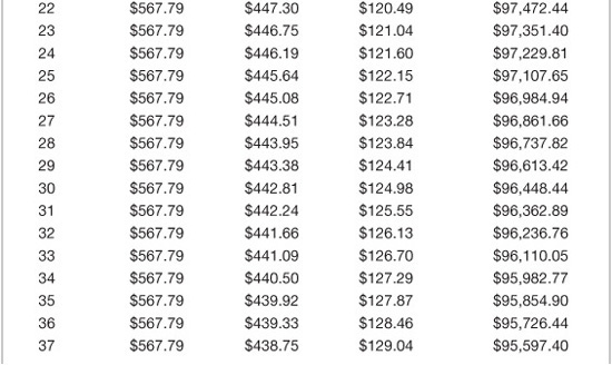
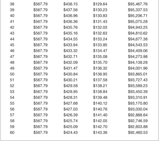
The exhibit shows that the payment consists mostly of interest in the early period of the loan. Since interest is calculated from a progressively declining balance and the aggregate payment is fixed, the amount of interest paid steadily declines; conversely, the principal component consequently increases over time. In fact, the exhibit shows that the unpaid principal balance in month 60 is $92,460, which means that of the $34,067 in payments made by the borrower to that point, only $7,539 was composed of principal payments. However, as the loan ages, the payment is increasingly allocated to principal. The crossover point in the example (i.e., where the principal and interest components of the payment are equal) comes in month 210. A graphic representation of principal and interest payments, along with the balance of the loan, is shown in Exhibit 24–2.
EXHIBIT 24–2
Allocations of Principal and Interest Payments for a $100,000 30-Year Fixed-Rate Loan with 5.5% Note Rate (Total Monthly Payment of $567.79)
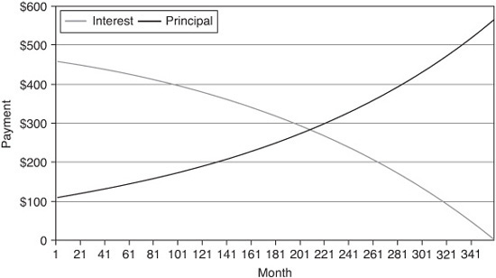
Loans with shorter amortization schedules (e.g., 15-year loans) allow the buildup of equity in the home at a much faster rate. Exhibit 24–3 shows the outstanding balance of a $100,000 loan with a 5.5% note rate using 30- and 15-year amortization terms. Note that while 50% of the 30-year loan balance is paid off in month 246, the halfway mark is reached in month 151 with a 20-year term and month 107 with a 15-year loan. The chart also shows the outstanding balance for a 30-year loan with a 10-year interest-only period. In the case of balloon loans, the monthly payments are calculated to amortize the principal balance over a 360-month term. The balloon payment occurs at either month 60 (for a five-year balloon) or month 84 (for a seven-year balloon) and refers to the unpaid principal balance at the balloon date.
EXHIBIT 24–3
Unpaid Principal Balance for a $100,000 Fixed-Rate Loan at 5.5% for Different Loan Terms and Amortization Schemes
For an amortizing ARM loan, the payment is calculated at the initial note rate for the full 360-month term. At the first reset and at every subsequent adjustment, the loan is “recast,” and the monthly payment schedule is recalculated using the new note rate and the remaining term of the loan. For example, the payments on a three-year hybrid ARM with a 4.5% note rate initially would be calculated as a 4.5% loan with a 360-month term. If the loan resets to a 5.5% rate after three years, the payment is calculated using a 5.5% note rate and a 324-month term. The following year, the payment would be recalculated again using the prevailing rate (depending on the performance of the index referenced by the loan) and a 312-month term.
In general, mortgage loans can be prepaid at the option of the borrower. When a loan is prepaid, the holder of the loan (either in the form of a loan in portfolio or as part of a mortgage-backed security) receives the prepaid principal at face value. Prepayments take place for a variety of reasons. They may occur when a borrower “refinances” the loan, sells the underlying property, or defaults on the loan. Prepayments (especially those due to refinancing) hurt the holder of the mortgage by calling away the asset and forcing the holder to reinvest the proceeds at lower interest rates. The causes and implications of prepayments are discussed in more depth below.
THE MORTGAGE INDUSTRY
Within the mortgage market, there are a number of different types of financial institutions involved, either directly or indirectly, in the business of making mortgage loans. A number of different classification schemes can be used to distinguish businesses and functions.
Direct versus Third-Party Originations
As indicated by the nomenclature, a direct lender actually underwrites and funds loans. Conversely, a mortgage broker represents clients and typically works through multiple lenders to obtain financing for borrowers. The broker does not, however, either make the underwriting decision or fund the loan in such “third-party” originations or TPOs, but rather serves as an agent linking borrowers and lenders. Many large lenders divide their operations into units or channels that deal with TPOs (generally called the wholesale channel) along with those that work directly with borrowers (the retail channel). These distinctions are necessary partly because the different channels have differing cost structures, necessitating alternative pricing.
Depository versus Nondepository
Depository institutions (which include banks, savings and loans, and credit unions) collect deposits from both wholesale and retail sources and use the deposits to fund their lending activities. Since depositories have portfolios (for both loans and securities), they have the option of either holding their loan production as a balance sheet asset or selling the securitized loans into the capital markets in the form of mortgage-backed securities (MBS). (In addition, there is a market for nonsecuritized mortgage portfolios among depositories because there are accounting advantages to holding loans on their books instead of securities.) Nondepository lenders (mainly so-called mortgage bankers) do not have loan portfolios; virtually all their loan production is sold to investors through the capital markets. (This is sometimes referenced as the “loans-to-bonds” business model.) Depositories that can hold mortgages or MBS in portfolio sometimes can be more aggressive in how they price different products, especially products they wish to accumulate in their loan or investment portfolios (most frequently short-duration assets such as adjustable-rate loans). By contrast, mortgage bankers must price all their production based on capital markets execution. This means that mortgage bankers are at a competitive disadvantage in issuing products for which capital market demand is either weak or nonexistent; they may also find it difficult at times to compete in some product sectors targeted aggressively by banks.
Originators versus Servicers
Loan originators underwrite and fund loan production. However, once a loan is closed, an infrastructure is required for collecting and accounting for principal and interest payments, remitting property taxes, dealing with delinquent borrowers, and managing the process of foreclosing on nonperforming loans. Entities that provide these functions are called servicers. For providing these services, such entities receive a fee, which generally is part of the monthly interest payment. Servicing as a business is both labor- and data-intensive. As a result, large servicing operations reap the benefit of economies of scale under normal industry conditions (i.e., when delinquencies are relatively low.) However, such large servicers are poorly prepared to deal with large numbers of seriously delinquent loans. During 2010, this led to a serious backlog in the handling of nonperforming loans, as well as controversy surrounding the practices and activities of a number of large servicers.
Servicing as an asset may be classified along several dimensions. Required, or “base,” servicing is compensation for undertaking the activities described earlier, and is either dictated by industry guidelines or (in the case of nonagency securities or loans) conditional on the product. For example, as of this writing, lenders must hold 25 basis points of base servicing for fixed-rate loans being securitized into GSE-eligible pools, whereas Ginnie Mae requires either 19 or 44 basis points (depending on the securitization vehicle) for similar loans. The ownership of base servicing also provides the servicer with ancillary benefits, including interest float on insurance and tax escrow accounts, along with the ability to cross-sell other products using the database of borrower information. “Excess” servicing is any additional servicing over the base amount and is merely a strip of interest payments held by the servicer that allows the loan to be securitized with an “even” coupon, as demonstrated later in the section on execution dynamics. Excess servicing neither requires any activity on the part of the servicer nor does it convey any benefits; it is strictly a by-product of the securitization process.
The Loan Underwriting Process
After the application for a loan is filed, it is considered to be part of the “pipeline,” which suggests that there is a planned sequence of activities that must be completed before the loan is funded. At application, the borrower can either lock the rate of the loan or let it float until some point before the closing. From the perspective of the lender, there is no interest-rate risk associated with the loan until it is locked. However, after the loan is locked, the lender is exposed to risk in the same fashion as any fixed-rate asset. Lenders typically track locked loans and floating liabilities separately; they are referred to as the “committed” versus the “uncommitted” pipeline.
There are two essential and separate components of the underwriting process:
• Evaluation of the ability and willingness on the part of the borrower to repay the loan in a timely fashion
• Ensuring the integrity of the property and whether it can be sold in the event of a default to pay off the balance of the loan
There are several factors that are considered important in the evaluation of the creditworthiness of a potential borrower.
Credit Scores
Several firms collect data on the payment histories of individuals from lending institutions and use sophisticated models to evaluate and quantify individual creditworthiness. The process results in a credit score, which is essentially a numerical grade of the credit history of the borrower. There are three different credit reporting firms that calculate credit scores, namely Experian (which markets the Experian/Fair Isaac Risk model), Transunion (which supports the Emperica model), and Equifax (which calls its model Beacon). While the credit scores have different underlying methodologies, the scores generically are referred to as “FICO scores.” Lenders attempt to obtain more than one score in order to minimize the impact of variations in credit scores across providers. In such cases, if the lender obtains all three scores, generally the middle score is used, whereas the convention is to use the lower value in the case of the availability of only two scores.
Credit scores are useful in quantifying the potential borrower’s credit history. The general rule of thumb has traditionally been that a score in excess of 700 represents a “strong” borrower. The problems associated with the financial crisis led to a reassessment of this threshold; a 730 or higher score is currently considered necessary for borrowers to receive the best rates and offerings from lenders.
Loan-to-Value Ratio
The loan-to-value ratio (LTV) is an indicator of a borrower’s leverage at the point when the loan application is filed. The LTV calculation compares the value of the desired loan to the market value of the property. By definition, in a purchase transaction a loan’s LTV is a function of the down payment and the purchase price of the property (subject to an appraisal). In a refinancing, it depends on the requested balance of the new loan and the appraised market value of the property.2 LTV is important for a number of reasons. First, it is an indicator of the amount that can be recovered from a loan in the event of a default, especially if the value of the property declines. It also has an impact on the expected payment performance of the obligor because high LTVs may indicate a greater likelihood of default on the loan. While loans can be originated with very high LTVs, borrowers seeking a loan with an LTV greater than 80% generally must obtain insurance for the portion of the loan that exceeds 80%. As an example, if the borrower applies for a $90,000 loan in order to buy a property for $100,000, he or she must obtain so-called mortgage insurance (MI) on $10,000 of the balance. Mortgage insurance is a monthly premium that is added to the loan payment and can be eliminated if the borrower’s home appreciates (or the loan is paid down) to the point where the loan has an LTV below 80%.
Another measure used by underwriters is the combined LTV (CLTV), which accounts for the existence of any second liens. A $100,000 property with an $80,000 first lien and a $10,000 second lien will have an LTV of 80% but a CLTV of 90%. For the purposes of underwriting a loan, CLTVs are more indicative of the borrower’s credit standing and indebtedness than LTVs and therefore a better gauge of the creditworthiness of the loan.3
Income Ratios
In order to ensure that borrowers’ obligations are consistent with income, lenders calculate debt-to-income (or DTI) ratios that compare the potential monthly payment on the loan to the borrower’s monthly income. The most common measures are front and back ratios. The front ratio is calculated by dividing the total monthly payments on the home, including principal, interest, property taxes, and homeowners insurance, by the borrower’s pretax monthly income. The back ratio is similar but adds other debt payments (including auto loan and credit card payments) to the total payments. The traditional limits for front and back ratios are 28% and 36%, respectively.
Documentation
Lenders traditionally have required potential borrowers to provide data on their financial status and to support the data with documentation. Loan officers typically require applicants to report and document income, employment status, and financial resources (including the source of the down payment for the transaction). Part of the application process routinely involves compiling documents such as tax returns and bank statements for use in the underwriting process. In the period between 2000 and 2007, however, documentation standards were progressively relaxed, leading to the proliferation of limited- and no-documentation loan programs. Popular options included “stated income” loans (which required borrowers to supply an income figure but did not require supporting documentation) as well as programs that required no disclosures of incomes, assets, or employment. (These programs were often labeled “no income/no asset” or “NINA” loans.)
The trend began in the mid 1900s with programs targeted to borrowers whose credit was sound but who had income streams that were either variable or, in the case of self-employed borrowers, difficult to document. This eventually led to the widespread marketing of loans to wage earners who often used the absence of formal documentation to inflate their incomes and evade DTI analysis.
One result of the financial crisis that began in 2007 was the return of rigorous underwriting standards, with full income and asset documentation a key requirement. While this certainly strengthened the credit quality of loans issued under this regime, it unfortunately also served to shut many otherwise strong borrowers out of the mortgage and housing markets due to difficulties in documenting their incomes.
GENERATION OF MORTGAGE LENDING RATES
While it may appear simple on the surface, the determination of mortgage lending rates is a complex interplay between levels in the secondary market for loans (or, more typically, MBS), the value of servicing, the cost of credit enhancement, and the costs associated with generating the loan. In this process, the pricing of different MBS (quoted directly and through the mechanism of intercoupon spreads) is very important in determining the eventual disposition of loans. The MBS market serves to institutionalize the intermediation function by allowing providers of funds (investors) and users of funds (lenders) to interact at the national level. Using the MBS market, lenders make loans, package them into securities, sell them into the capital markets, and use the proceeds to make new loans. While certain lenders may hold some loans and products in loan portfolios (e.g., banks tend to hold short-duration products such as ARMs), the bulk of production is securitized and sold into the capital markets.
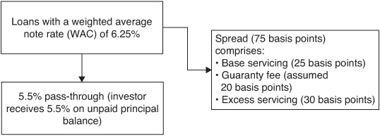
While a complete discussion of the MBS market is beyond the scope of this chapter, it is instructive to review the process involved in securitizing loans because of the importance of this process in the determination of lending rates. For the sake of simplicity, the following discussion focuses on fixed-rate conforming loans securitized through the GSE programs. The coupons on such pools (or “pass-throughs” because they pass principal and interest through to the investor) generally are created in ½ percentage point increments, e.g., 5.5%, 6.0%, etc. Loans, by contrast, generally are issued in ![]() percentage point increments. The creation of pools to be traded as MBS involves the aggregation of loans with similar characteristics, including note rates that are a minimum and maximum amount over the coupon rate, depending on the agency and program. The weighted average of the note rates of the loans in the pool is referred to as the pool’s “weighted average coupon” (WAC). The spread between the pool’s WAC and its coupon rate (or pass-through rate) is allocated to three sources:
percentage point increments. The creation of pools to be traded as MBS involves the aggregation of loans with similar characteristics, including note rates that are a minimum and maximum amount over the coupon rate, depending on the agency and program. The weighted average of the note rates of the loans in the pool is referred to as the pool’s “weighted average coupon” (WAC). The spread between the pool’s WAC and its coupon rate (or pass-through rate) is allocated to three sources:
• Required or base servicing, which refers to a portion of the loan’s note rate that is required to be held by the servicer of the loan. As noted previously, this entity collects payments from mortgagors, makes tax and insurance payments for the borrowers, and remits payments to investors. The amount of base servicing required differs depending on the agency and program.
• Guaranty fees (or “g-fees”) are fees paid to the agencies to insure the loan. Since these fees essentially represent the price of credit risk insurance, there is variation across loan types. In the conventional universe, loans that are perceived to be riskier typically require a higher g-fee for securitization. For Ginnie Mae pools, the guaranty fee is almost always 6 basis points. Note that for Fannie Mae and Freddie Mac securities, g-fees can be capitalized and paid as an upfront fee in order to facilitate certain execution options.
• Excess servicing is the remaining amount of the note rate that would reduce the interest rate of the loan to the desired coupon. This asset generally is capitalized and held by the servicer. Nonetheless, secondary markets exist for trading servicing in the form of either raw mortgage servicing rights or securities created from excess servicing.
A schematic showing how a typical pool issued by the GSEs allocates cash flows is shown in Exhibit 24–4.
EXHIBIT 24–4
Cash-Flow Allocation for a 5.5% GSE Pass-Through Pool
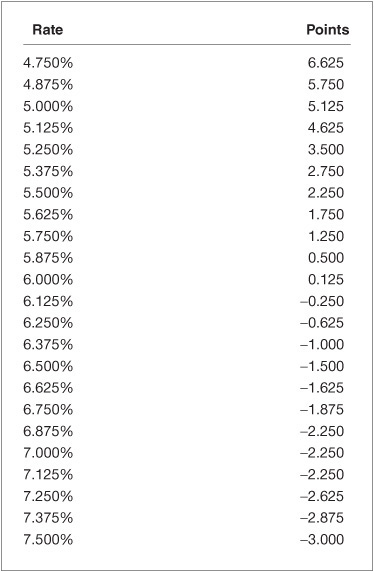
A common misconception is that lenders quote rate levels to consumers. In actuality, lenders calculate “discount points” (i.e., an up-front fee paid at closing) for a broad range of note rates. Note that these rate levels can be associated with both positive and negative points. (Negative points can be thought of as a rebate to the borrower in exchange for paying a higher rate.) The process for other products is similar in concept, if not identical in process. Exhibit 24–5 shows a hypothetical matrix of rates and points for 30-year conforming fixed-rate loans.
EXHIBIT 24–5
Hypothetical Rate/Point Matrix for 30-Year Conforming Fixed-Rate Loans
Given existing market conditions, the process of generating points involves two steps:
• Determining the optimal execution for each note rate;
• Calculating the appropriate amount of points for each note rate.
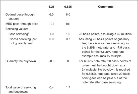
Loans can be securitized in pools with a wide range of coupons (e.g., a conventional loan with a 6.5% note rate can be securitized in Fannie Mae or Freddie Mac pools with coupons ranging from 4.0% to 6.25%). To maximize their proceeds, the optimal execution is calculated regularly by the originator and is a function of the levels of pass-through prices, servicing valuations, and guaranty fee buydown proceeds.4 Exhibit 24–6 shows two possible execution scenarios for a loan with a 6.25% note rate. Note that execution economics generally dictate that loans are pooled with coupons between 25 and 75 basis points lower than the note rates; creating a larger spread between note rate and coupon normally is not economical. In the example, securitizing the loan in the 6.0% pool is the best execution option because it provides the greatest proceeds to the lender.
EXHIBIT 24–6
Pooling Options for a 6.25% Note Rate Loan Using Hypothetical Prices and Levels
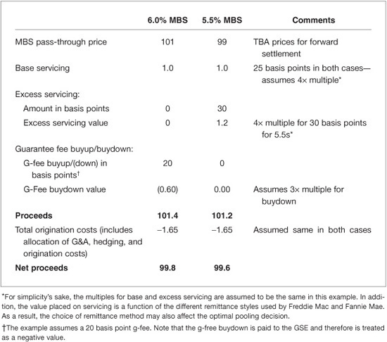
Once the optimal execution is determined for each note rate strata, the associated points are then calculated. As with the execution calculation, the calculation of points is based on market prices for pass-throughs and prevailing valuations for servicing and g-fee buydowns. Exhibit 24–7 shows a hypothetical calculation of points for loans with 6.25% and 6.625% note rates, assuming that the best execution for both rates would be securitized as part of pools with a 6.0% coupon rate. The calculated points are shown at the bottom as the difference between the net value of the loan after pricing all components and its par value. While the example does not show it, points generally are rounded to the nearest one-eighth. In practice, points are calculated simultaneously for many rate levels and are subsequently posted in a rates/point matrix similar to the one shown in Exhibit 24–7.
EXHIBIT 24–7
Sample Calculation of Points Given a Lending Rate (All Levels Hypothetical)
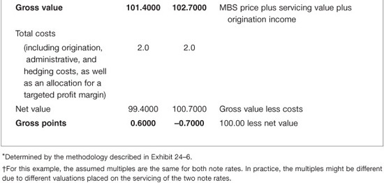
Note also that the costs shown in Exhibit 24–7 include an allocation for the lender’s targeted profit margin. Margin requirements change in line with market conditions, most notably based on the levels of lending volumes and the industry’s price competitiveness at that time.
In the event that the loan is perceived to be riskier as a result of factors that may include a lower credit score, less documentation, and/or a higher LTV, it would be assigned a higher guaranty fee by the GSE. As a result, the loan would be more costly to the borrower. As an example, assume that the 6.25% note rate loan shown in Exhibit 24–7 was assigned a 30-basis points guaranty fee. At the 3× multiple, the guaranty fee buydown cost is 0.9. The incremental 0.3 cost of credit enhancement means that the loan’s net value is 99.1; the 6.25% loan would therefore be priced to have 0.9 points. Therefore, the lending paradigm called risk-based pricing means that the higher costs (in the form of points at a given note rate strata) associated with riskier loans represent greater credit enhancement costs that are being passed on to the borrower.
As mentioned, the examples show the calculation for a loan that is eligible to be securitized in a pool issued by one of the GSEs. If the loan were ineligible for such securitization, the cost of the guarantee fee is replaced by the cost of alternative credit enhancement needed to securitize the loan. The most common form of credit support in nonagency transactions is called subordination. Briefly, this means that bonds created within the deal are prioritized with respect to how they will receive principal and interest cash flows, as well as how they will accrue losses suffered by the transaction’s collateral pool. (Higher-priority or more senior bonds have the highest priority for receiving cash flows, and are the last to suffer writedowns.) As a result, the cost of credit enhancement to the transaction is a function of two elements:
• The relative size of the subordinate or junior classes of bonds;
• The price at which they can be sold to investors.
The size of the subordinate classes has traditionally been assigned by the rating agencies. Their primary role is to determine how large the subordinates need to be in order for the senior bonds to receive a triple-A rating. In turn, the size of the subordinate classes is a function of the perceived riskiness of the loans backing the transaction. The level at which the subordinates trade in the new-issue market is dictated by the price at which investors feel they can garner attractive risk-adjusted returns. Subordinates typically trade at large price discounts to the more senior bonds in order to account for their greater risks and/or reduced protection from losses.
Therefore, the cost of credit support in non-agency or private-label transactions is expressed by the weighted average price at which the subordinate classes can be sold. Riskier collateral thus has higher credit enhancement costs, since the amount of subordination is higher and/or the overall price at which the subordinates can be sold is lower.
Risk-based pricing is accomplished in two ways. Lenders often create separate loan programs that reflect a set of attributes, and price the program based on the loans’ credit enhancement costs. This was reflected in the proliferation of different lending programs prior to the financial crisis. In cases where creating a separate program is inefficient or undesirable, attributes are priced using “add-ons,” or points added to the discount points calculated in the manner described previously. Add-ons (often called Loan-Level Price Adjustments, or LLPAs) are fees calculated to account for the incremental cost of credit enhancement for a loan. Similar to discount points, such fees are quoted as percentage points of the loan’s face value. For example, a 30-year fixed-rate conforming-balance loan with a 5.875% note rate may be associated with ½ point. However, a borrower may seek a loan with an LTV higher than that specified by the program’s guidelines. If the add-on in this case is 1½ points, the loan then becomes a 5.875% loan with 2 points.
However, the disinclination of many borrowers to paying large amounts of money at closing necessitates a recalculation of the rate, given some targeted amount of points and the rate/point structure prevailing at that time. In the preceding example, suppose that the borrower only wishes to pay ½ point after the effect of the add-ons. Referring to Exhibit 24–5, note that a loan with ½ point is associated with a 5.875% note rate, whereas a loan with negative 1 point has a note rate of 6.375%. Therefore, the borrower in the example could obtain a loan with a rate of 6.375% with ½ point. This methodology indicates how the expense, calculated in terms of points, of “alternative” loans is translated into incrementally higher note rates.
COMPONENT RISKS OF MORTGAGE PRODUCTS
Holders of fixed income investments ordinarily deal with interest-rate risk, which is the risk that changes in the level of market interest rates will cause fluctuations in the market value of such investments. Mortgages and associated mortgage-backed securities, however, have additional risks associated with them that are unique to the products and require additional analysis. (In the following discussions, mortgages and MBS are collectively referred to as pools for the sake of clarity.)
Prepayment Risk
In a previous section we noted that obligors generally have the ability to prepay their loans before they mature. For the holder of a mortgage asset, the borrower’s prepayment option creates a unique form of risk. In cases where the obligor refinances the loan in order to capitalize on a drop in market rates, the investor has a high-yielding asset payoff, and it can be replaced only with an asset carrying a lower yield. Prepayment risk is analogous to “call risk” for corporate and municipal bonds in terms of its impact on returns, and it also creates uncertainty with respect to the timing of investors’ cash flows. In addition, changing prepayment “speeds” owing to interest-rate moves cause variations in the cash flows of mortgage pools, strongly influencing their relative performance.
The importance of prepayments to the mortgage sector has created the need for the measurement and analysis of prepayment behavior. Prepayments occur for the following reasons:
• The sale of the property;
• The destruction of the property by fire or other disaster;
• A default on the part of the borrower (net of losses);
• Curtailments (i.e., partial prepayments); and
• Refinancing.
A useful nomenclature is to divide prepayments into “rate-sensitive” and “rate-insensitive” categories. Rate-insensitive prepayments traditionally have been comprised of housing turnover, which normally consists of home sales, along with equity extraction through the vehicle of cash-out refinancings. The spike in delinquencies and credit problems after 2007, however, meant that credit-related prepayments also needed to be taken into account in assessing prepayment speeds. (Since mid 2010, for example, the GSEs are forced to buy seriously delinquent loans out of pools. Such buyouts are treated as prepayments in agency pools. As we will discuss, credit-related prepayments are treated differently in private-label securities.)
Rate-sensitive prepayments primarily consist of refinancings for which borrowers do not monetize their homes’ equity, and are also called “rate-and-term” refinancings. This activity is dependent on borrowers’ ability to obtain a new loan at a lower rate, making this activity highly sensitive to the level of interest and mortgage rates. In addition, the amount of refinancing activity can change greatly given a seemingly small change in rates. The paradigm in mortgages thus is fairly straightforward. Mortgages with low note rates (that are “out-of-the-money,” to borrow a term from the option market) normally prepay fairly slowly and predictably, whereas loans carrying higher rates (“in-the-money”) can see spikes in prepayments when rates drop, as well as significant volatility in prepayment speeds.
The measurement of prepayment rates is, on its face, fairly straightforward. A metric referred to as single monthly mortality (SMM) measures the monthly principal prepayments on a mortgage portfolio as a percentage of the balance at the beginning of the month in question. (Note that SMM does not include regular principal amortization.) The conditional prepayment rate (CPR) is simply the SMM annualized using the following formula:
CPR = 1 – (1 – SMM)12
While CPR is the most common term used to describe prepayments, other conventions are also used. Logic suggests, for example, that prepayment behavior is not constant over the life of the loan. Immediately after the loan is funded, for example, a borrower is unlikely to prepay his mortgage; however, the propensity to prepay (for any reason) increases over time. This implies that prepayments adhere to some sort of “ramp,” where the CPR increases at a predictable rate. The most common ramp is the so-called PSA model, created by the Public Securities Association (now called the Securities Industry and Financial Markets Association, or SIFMA). The base PSA model (100% of the model or 100% PSA, to use the market convention) assumes that prepayments begin at a rate of 0.2% in the first month and increase at a rate of 0.2% per month until they reach 6.0% CPR in month 30; at that point, prepayments remain at 6% CPR for the remaining term of the loan or security. Based on this convention, 200% PSA implies that speeds double that of the base model (i.e., 0.4% in the first month ramping to a terminal speed of 12% CPR in month 30.) Exhibit 24–8 shows a graphic representation of the PSA model.

The PSA model depends on the age of the loan (or, in a pool, the weighted-average loan age). For example, 4.0% CPR in month 20 equates to 100% PSA, whereas 4.0% CPR in month 6 represents 333% PSA. Conversely, the usefulness of the PSA model (or other ramps that are similar in nature) depends on how quickly prepayments move toward a terminal rate (or, to put it differently, how quickly they “ramp up”). It is generally understood that prepayment ramps have shortened since the model was derived, reflecting the lowering of refinancing barriers and costs. In turn, this arguably has distorted the reported PSA speeds for loans that are 30 months old or less, making the PSA model less useful as a measure of prepayment speeds.
While a full discussion of prepayment behavior and risk is far beyond the scope of this chapter, it is important to understand how changes in prepayment rates affect the performance of mortgages and MBS. Since prepayments increase as bond prices rise and market yields are declining, mortgages shorten in average life and duration when the bond markets rally. As a result, the price performance of the mortgage portfolio or security tends to lag that of bonds without prepayment exposure when interest rates decline. Conversely, prepayments tend to slow when market yields are rising, causing the average life and duration of the mortgages or MBS to increase. This phenomenon, generally described as extension, causes the price of the mortgage or MBS to decline more than comparable fixed-maturity instruments (such as Treasury notes) as the prevailing level of yields increases.
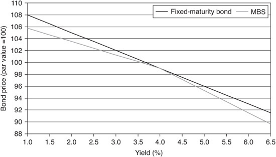
Owing to changes in prepayment rates, mortgages and MBS exhibit price performance that is generically referenced as “negative convexity.” Since prepayments increase when rates decline, MBS shorten in average life and duration at precisely the time when their performance would benefit from extending. Conversely, when the bond market sells off, mortgage average lives and durations lengthen. This behavior causes the price changes in mortgages and MBS to be decidedly nonlinear in nature and to underperform those of assets that do not exhibit negatively convex behavior. Exhibit 24–9 shows a graphic representation of this behavior. Investors are generally compensated for the lagging price performance of MBS through higher base-case yields. However, the necessity of managing negative convexity and prepayment risk on the part of investors dictates active analysis and management of their MBS portfolios.
EXHIBIT 24–9
Performance Profile of Hypothetical Fixed-Maturity Bond versus MBS
Credit and Default Risk
Analysis of the credit exposure in the mortgage sector is different from the assessment of credit risk in most other fixed income instruments because it requires:
• Quantifying and stratifying the characteristics of the thousands of loans that underlie the mortgage investment;
• Estimating how these attributes will translate into performance based on standard metrics and the evaluation of reasonable best-, worst-, and likely-case performance;
• Calculating returns based on these scenarios.
In a prior section, some of the factors (credit scores, LTVs, etc.) that are used to gauge the creditworthiness of borrowers and the likelihood of a loan to result in a loss of principal were discussed. Many of the same measures are also used in evaluating the creditworthiness of a mortgage pool. For example, weighted-average credit scores and LTVs are calculated routinely, and stratifications of these characteristics (along with documentation styles and other attributes) are used in the credit evaluation of the pool. In addition to these characteristics of the loans, the following metrics are also relevant for the a posteriori evaluation of a mortgage pool.
Delinquencies
Delinquency measures are designed to gauge whether borrowers are current on their loan payments or, if they are late, stratifying them according to the seriousness of the delinquency. The most common convention for classifying delinquencies is one promulgated by the Office of Thrift Supervision (OTS); this OTS method classifies loans as follows:
• Payment due date to 30 days late: Current
• 30–60 days late: 30 days delinquent
• 60–90 days late: 60 days delinquent
• More than 90 days late: 90+ days delinquent
Defaults
At some point in their existence, some delinquent loans become current (or cure) because the condition leading to the delinquency (e.g., job loss, illness, etc.) resolves itself. However, some portion of the delinquent loan universe ends up in default. By definition, default is the point where the borrower loses title to the property in question. Default generally occurs for loans that are 90+ days delinquent, although loans where the borrower goes into bankruptcy may be classified as defaulted at an earlier point in time.
It is important to note that the treatment of defaults in agency and nonagency securities is different. As noted in the previous section, seriously delinquent loans are bought out of agency pools. Since the agency in question is responsible for the repayment of the full amount of principal to investors, buyouts are prepayments for all practical purposes. No such mechanism exists for private-label securities; principal is only paid to investors once it is recovered through the foreclosure process (or through some alternative mechanism, such as a short sale.) Moreover, only the recovered amount of principal is returned to investors, with the transaction absorbing the resulting losses.
Therefore, defaults in private-label transactions must be treated and quoted separately from refinancings, turnover, and other types of voluntary prepayments. Rates for involuntary prepayments are generally measured by the conditional default rate, or CDR. CDRs are calculated in a fashion similar to CPRs, in which the face value of loans going into default in any given month is divided by that month’s initial value. The resulting monthly default rate (or MDR) is then annualized in the same fashion as SMMs.
Severity
Since the lender has a lien on the borrower’s property, some of the value of the loan can be recovered through the foreclosure process. Loss severity measures the face value of the loss on a loan after foreclosure is completed. Severities are often heavily influenced by the loan’s LTV (since a high LTV loan leaves less room for a decline in the value of the property in the event of a loss). However, in the event of a default, even loans with relatively low LTVs can experience significant losses, generally for several reasons:
• The appraised value of the property may be high relative to the property’s actual market value.
• The value of a property may have declined since the loan’s origination due to changes in the real estate market.
• There are costs and lost income associated with the foreclosure process.
In light of these metrics, the process of evaluating the credit-adjusted performance of a pool involves first understanding the expected delinquencies, defaults, and loss severities of the pool based on its credit characteristics and attributes. Subsequently, loss-adjusted yields and returns can be generated.
KEY POINTS
• Mortgage loans can be categorized using a number of different factors, including: lien status; original loan term, interest-rate type, balance classification, amortization type, and borrower credit and documentation standards. Loans can also be categorized by the type of credit support they receive, i.e., guarantees directly from the U.S. government, through Freddie Mac or Fannie Mae, or some form of private credit enhancement.
• The payments on a fixed-rate fully amortizing mortgage remain fixed for the term of the loan. Early in a loan’s life, the bulk of the payments are classified as interest. However, the portion directed to repay principal grows as the loan ages.
• Mortgage underwriting is a complex process that takes into account borrowers’ ability and apparent willingness to service their loans. These are judged using metrics such as credit scores, loan-to-value ratios, and income ratios. The accurate documentation of income, employment, and assets has also proved to be important in assessing borrower creditworthiness.
• Mortgage lenders calculate their pricing in the form of the discount points required or rebated for a series of note rate strata. Consumer mortgage pricing is computed through a complex process that incorporates MBS levels, servicing values, and the cost of credit support.
• Securities backed by residential mortgages have a variety of risks. In addition to interest rate risk, mortgage-backed securities are exposed to prepayment risk, as well as credit risk if the securities in question do not have explicit or implicit government backing.