
CHAPTER
TWENTY-SIX
AGENCY COLLATERALIZED MORTGAGE OBLIGATIONS
This chapter provides an introduction to the U.S. agency collateralized mortgage obligation (CMO) market. It begins with the background of the CMO market and explains the difference between agency and nonagency CMOs. The chapter introduces the issuers Fannie Mae, Freddie Mac, and Ginnie Mae, then covers all of the major CMO tranche types in terms of structure and analysis, providing practical examples. It also covers information about option-adjusted spread (OAS) and prepayment models, and how to use that information to hedge CMOs or determine relative value. Coverage of nonagency CMOs is provided in Chapter 31.
THE CMO MARKET
The CMO market has existed since the mid 1980s. Its original purpose was to allow investors to more closely control when they receive principal from mortgage backed securities. With mortgage pass-throughs, principal is received each month throughout the life of a security, often for a full 30 years. In a CMO, the principal is divided up into pieces or “tranches” creating some bonds that receive principal right away (and hence have shorter durations) and bonds that do not, typically resulting in longer durations. The creation of so-called PAC, or planned amortization class bonds took the CMO a step further, attempting to create a corporate bond surrogate.
To create a CMO, a dealer must gather agency pass-through collateral, structure a deal, then pay a fee to Freddie Mac, Fannie Mae, or Ginnie Mae to issue the CMO. Ginnie Mae has the full faith and credit of the U.S. Government, whereas the other agencies have the implicit guarantee of the U.S. Government.
Now, the CMO market has exploded into a myriad array of tranches using different types of collateral. The cash-flow priority of tranches can even jump around based on prepayments. The same financial technology used to create CMOs has been employed to create other securitized products in the world global market.
This chapter was written when the author was an employee of Deutsche Bank.
When comparing nonagency CMOs to agency CMOs, agency CMO analysis tends to be simpler because of more established prepayment models and minimal credit risk. Collateral information disclosure on nonagency CMOs tends to be slightly better, but in general the information gap is marginal for new deals.
THE REASONS WHY CMOs EXIST
Like any security, CMOs exist because there is a market to buy and sell them. From the demand side, there are investors who still want to more closely control the cash flows they get from an MBS investment. In addition, the CMO market has grown to such an extent that many other things are possible using the CMO market than with the MBS pass-through market, such as bonds with coupons that adjust on a monthly basis (floaters). From the supply side, CMO originators continue to operate as long as they can make a reasonable profit in the business. Often, all the CMO tranches are not sold right away, which forces the dealer to hold inventory, and thus take risk.
Size of the CMO Market
Peak issuance of CMOs was over $1 trillion in 2005. CMO issuance dropped to only $191 billion during the financial crisis of 2008, but has since rebounded. For example, CMO issuance in 2010 exceeded $500 billion. Historically, issuance of new CMOs has surpassed that in most other markets, including Treasuries and corporate bonds.
Liquidity
The raw size of the CMO market suggests it should have enormous liquidity. However, liquidity is somewhat hampered by lack of homogeneity in the CMO market. Even the most common tranche types, PACs and sequentials, may have subtle differences that need to be examined and valued. (We will discuss this in detail later.) The liquidity of CMOs is typically less than pass-throughs, but comparable to corporate bonds. Even specialized derivatives, such as interest-only (IO) strips often have relatively tight bid/ask spreads of around an eighth of a point during normal market conditions.
Practical Details
In this section, we cover practical details such as typical payment and settlement structure for CMOs. Rules are generally different for CMOs than for corporate bonds. In some cases, rules are different for certain types of CMO tranches than for pass-throughs.
Bond Settlement
CMOs usually settle in book entry via DTC (Depository Trust Co.). Primary market CMOs may have delayed settlement, similar to pass-throughs. For example, many new-issue CMOs settle in the month after the trade date. New-issue CMOs usually settle at the end of the month, to allow the dealer time to bring in collateral and finish structuring the deal.
Secondary market CMO transactions are typically for corporate settlement, presently T+3 business days. It is possible to trade CMOs for other settlements, such as cash, if necessary.
Monthly Interest and Principal Payments
CMOs pay interest monthly, similar to the underlying pass-throughs. Tranches eligible to receive principal payments will receive them at the same time as the interest payments. Most CMOs have the same number of delay days as the underlying collateral, for example, 55 stated delay days for FNMA pass-throughs. However, certain tranches, such as CMO floaters, may have reduced delay days to facilitate comparison to corporate bonds. The number of delay days for each tranche is available in the prospectus or from electronic sources. Of course, the number of delay days impacts yield, as interest and principal are returned later (and hence reinvestment interest on that interest and principal is foregone) the longer the delay is.
Deal Clean-Up Calls
Some deals may contain clean-up calls triggered when only a small portion of the deal remains. The percentage trigger is typically set between 1% and 10%, inclusive. This feature is typically set up to avoid the burden of high fixed costs for the deal’s trustee when a small amount of bonds remains outstanding. We discuss analyzing deal clean-up calls later in this chapter.
New Issue versus Secondary Markets
The new issue CMO market typically settles as much as one or two months in the future, allowing the issuer to gather the requisite collateral for the deal and complete structuring. This structuring period also affords the investor the opportunity to custom design CMO tranches that fit into his portfolio. Most secondary tranches trade for corporate settlement. While the investor cannot change existing tranches, more information about the tranche, such as historical prepayment speeds, can be valuable to the investor.
CMO TRANCHE TYPES
The crux of understanding the CMO market is understanding the different tranche types and how they are structured. Today, CMO deals are very complex, with multiple collateral sources, multiple tranche types, etc. in a complex array for each CMO deal. It is important to realize that each of these deals is made primarily from two basic flavors.
• A planned amortization class (PAC) deal, in which the non-PAC (support or companion) tranches have highly variable cash flows and average lives, while the PAC enjoys relatively stable, prescheduled cash flows.
• A sequential deal, where standard sequential tranches have cash-flow priority (i.e., absorb most or all of the principal from the deal) in turn until they are all retired.
These types of deals can be altered or dressed up slightly (such as in a PACquential deal), but there are still two basic flavors. Once the PACs and sequentials are created, they can be divided even further (e.g., into a PAC floater and PAC inverse floater). It is also possible to add other tranches with special features, such as a tranche where interest accrues back into the principal, called a Z-bond (i.e., zero coupon). Nevertheless, to understand the structure of CMOs, one must always start with that first question on which deal type it is, then walk through how an individual tranche was created in order to correctly analyze it.
For each tranche type in this section, we will provide the following: description, example, yield table, and methods of analysis. Note that while we have tried to be as realistic as possible in showing yield table and OAS analysis for CMO tranches, these numbers do not necessarily correspond to anything available in the market currently. These examples have been constructed mainly for learning purposes, not to illustrate relative value or hedging purposes! We also do not identify deal names or CUSIPs on any of these bonds for those reasons.
Sequential
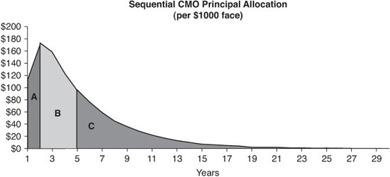
A sequential CMO, also historically referred to as a “vanilla bond,” deal typically takes the collateral’s principal and time tranches it. The first sequential tranche receives all of the prepaid and scheduled principal from the deal until the tranche is retired, then the next sequential in line starts receiving principal. For example, in a simple three-tranche sequential (Exhibit 26–1), the first sequential could be allocated 30% of the deal’s principal. All principal cash flows from the underlying collateral would pay down the first sequential tranche to a zero balance. Then, the second sequential would receive its principal, and finally the third. The purpose of this structure is twofold. Investors may want a shorter or longer duration than the underlying collateral. In addition, the period of time before which the second sequential receives any principal is known as lockout. This lockout feature may be valuable to some investors who do not want to receive (and possibly need to reinvest) principal for some period of time.
EXHIBIT 26–1
Cash Flows from a Three-Tranche Sequential Deal
Example
Sequential bonds will have a different duration, average life, and projected cashflow for each prepayment assumption tested. In many respects, they perform like the underlying collateral of the CMO deal. Increase prepayments, and sequentials shorten their average life and duration. A few differences between sequentials and collateral:
• The window of time principal is returned to the investor in a sequential is narrower than that for collateral.
• A sequential can be locked out from prepayments (i.e., the factor remains 1.0) for some period of time. Pass-throughs start to factor down from 1.0 as soon as they are created.
• The coupon on a sequential (or any other CMO bond) can be different from the underlying collateral. Most commonly, the coupon on the sequential is “stripped down” lower than the collateral in order to create bonds that trade at or below par.
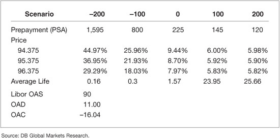
When a sequential coupon is stripped down, a portion of the interest from the collateral is diverted elsewhere in the deal.1 The purpose of this maneuver is to lower the price of the sequential bond, although typically the yield of the bond will also fall. Nomenclature in the CMO world talks of the tranche coupon versus the collateral coupon. For example, a 5.0/5.5 sequential would be a bond with a 5% coupon in a deal using 5.5% pass-through collateral.
Exhibit 26–2 compares the yield tables of a full coupon, 5.5/5.5 sequential with a stripped down 4.0/5.5 sequential. Note that the principal cash flows are essentially the same—the principal cash flows on these bonds react in the same way to changes in prepayment rates. However, market performance will likely be quite different, due to the longer duration of the 4.0/5.5 tranche. The 4.0/5.5 tranche has a 5.26 option-adjusted duration (OAD) versus a 3.11 OAD for the 5.5/5.5 full coupon sequential in our example. When interest (IO) is removed from a tranche, the negative duration associated with the IO is also removed, extending the duration of the remaining bond.
EXHIBIT 26–2
Comparing the Yield Tables of Full versus Stripped Down Coupon Sequentials

An intuitive way to think about premium and discount CMO durations is callable corporate bonds. As the price of the bond goes over par, it becomes harder for the price to rise given a drop in interest rates because of the call feature (in the case of MBS, faster prepayments). The duration of a high premium callable bond will be close to the call date because it is likely to be called. However, the duration of a deep discount callable bond is longer, close to the maturity date of the bond, because the bond is unlikely to be called.
Analysis
Analysis of sequentials falls into two broad categories:
• Analysis of short duration sequentials that are currently paying, typically as short duration bonds. They may be compared to short agencies, ABS, hybrid ARMs, other CMOs, etc.
• Longer duration sequentials that are often compared with the underlying collateral. Many characteristics of the sequential and collateral are typically similar: prepayment speeds, duration profile, etc.
For short duration bonds, investors are typically looking at yield and comparing it with similar duration bonds. In addition, investors need to evaluate the extension risk of the sequential to make sure it is not beyond their risk tolerance if interest rates rise, prepayment speeds slow, and the sequential extends.
For long duration bonds, comparison to collateral can be made using OAS or yield analysis, plus potentially a total rate of return analysis that compares expected returns of different bonds under different interest rate scenarios.
Planned Amortization Class
The second basic type of CMO deal is a PAC/support structure. PAC stands for planned amortization class and is one of the most stable classes of CMO. It is given a pre-set schedule for its principal pay down. If prepayment speeds were to remain at a fixed speed in a specific prepayment band (the PAC band) for the life of the security, the PAC would adhere to its original schedule and behave similarly to a corporate bond with a pro rata sinking fund structure. Exhibit 26–3 shows the amortization schedule for a hypothetical PAC.
EXHIBIT 26–3
Amortization Schedule for a Hypothetical PAC
PAC Bands, Band Drift, and Broken PACs
As mentioned, each PAC has a band, expressed in PSA terms. If prepayments remained constantly at that level throughout the life of the PAC, it would adhere to its planned amortization schedule and have the expected average life.
Of course, prepayments do not remain constant from month to month, let alone the life of a security. Therefore, over time, especially in a fast prepayment environment, the PAC bands on a PAC can drift, generally growing tighter over time (i.e., less advantageous for the investor).
One example of PAC band drift is in a fast prepayment environment. If approximately one-third of a PAC CMO deal is support bonds and prepayments increase over the top end of the PAC band, at some point, all the support bonds will be paid off. When the supports are gone, the PACs behave like sequential bonds, and are termed broken PACs in the marketplace. In reality, a broken PAC will behave like a sequential bond. However, due to the stigma of being “broken,” the broken PAC may trade more cheaply than a similar sequential.
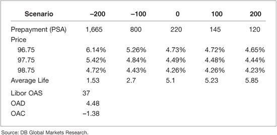
Exhibit 26–4 shows an example of a new PAC with a band of 100–250 PSA. Note that as interest rates rise, its average life stays around 5.95 years. However, since all MBS are inherently callable in any given month, very fast prepayment speeds engendered by a drop in mortgage interest rates cause the PAC to break out of its PAC band and shorten its duration significantly.
EXHIBIT 26–4
Example of a New PAC, Original PAC Band 100–250 PSA
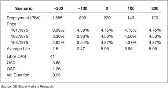
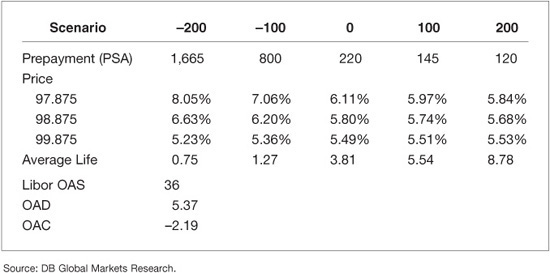
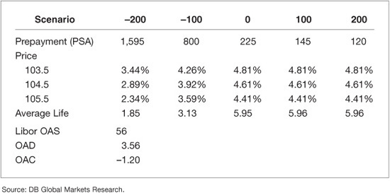
Exhibit 26–5, by contrast, shows a broken PAC originated a few years ago. All the support bonds in this deal have paid off, so it effectively behaves like a sequential. Note also that its OAS happens to be higher than the sequential bond analyzed earlier in this chapter. This can occur in the market if there is a glut of broken PACs. This bond currently does not have a PAC band left, but originally had a band of 100 to 255 PSA.
EXHIBIT 26–5
Example of a Broken PAC, no PAC Band Left

Analysis
The decision to buy PACs over sequentials or pass-throughs involves a couple of questions. First, is there a reason to buy cash-flow stability?
• Is cash-flow stability cheap via purchasing PACs?
• Is hedging pass-through or sequential cash flows using options or other derivatives expensive or cumbersome from an accounting perspective?
• Does the investor think the bond market is range-bound or could break out of its range?
• What do implied and actual volatility in the market look like and where are they going?
The answers to these questions can guide an investor toward whether to purchase PAC bonds.
Note that broken PAC analysis will be similar to sequential bond analysis. As mentioned, often broken PACs will trade at wider spreads than similar sequentials, creating relative value opportunities.2
Like sequentials, PACs can be compared using OAS analysis, yield, total return analysis, etc. with other MBS or even to corporate bonds because of the PACs’ stable nature.
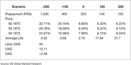
PAC 2
In some structures, the effectiveness of PAC classes is enhanced by creating a structure similar to a PAC, but with tighter PAC bands. In the priority of the cashflow waterfall, the PAC takes priority, followed by the PAC 2 (also referred to as Level II PACs and supports with schedules), and finally the support bonds. If the support bonds are retired and PACs remain, then the PAC 2s effectively become the new support bonds.
In return for the higher cash-flow variability of the PAC 2, it will yield more than similar PACs in the same deal. At the same time, in extreme prepayment environments, the PAC 2 will suffer extension or call risk before the PAC. The PAC 2 bond selected for Exhibit 26–6 has a relatively tight PAC band—so tight we cannot observe cash-flow stability on this bond in the ± 100 bp scenarios.
EXHIBIT 26–6
Example of a PAC 2, No PAC Band Remaining
Analysis
PAC 2 analysis needs to be very careful, as bonds from this class exhibit much more variability of structure, cash flows, and value than the PAC 1 or sequential tranche types. OAS analysis can help an investor make a determination if a bond is attractive. Investors also need to focus on potential duration extension and shortening in radical interest rate scenarios to make sure that duration change is tolerable. In our example bond, duration extension if rates rise is worse than with our example sequential bond.
Support Bonds
The support or companion bonds take whatever principal is left over each month after the PAC bonds have been paid as closely to schedule as possible. If prepayment speeds are fast, excess principal will pay down support tranches once planned principal payments to the PACs have been made. On the other hand, if prepayment speeds are very slow, all of the principal may go to the PAC bonds, with the support bonds receiving no principal for that month.
Example
The structuring of the support bond, with approximately 30% of a deal being companions and the balance PACs, makes for highly variable cash flows and a wide variety of performance characteristics. Because of this, companion yields tend to be quite high. Exhibit 26–7 shows how the average life of the bond can vary widely.
EXHIBIT 26–7
Example of a Support Bond
Analysis
Structures are very deal specific, and OAS models can help determine relative value among support bonds. Note however, that OAS and hence relative value will be very sensitive to model assumptions. Discount companions are more popular because they can be sold to retail investors more easily. Exhibit 26–7 shows our example companion, with high average life variability, but a big OAS. Note also that the structure and price prevents the yield of the bond from falling much below 6%, even in a rising interest rate environment. The yield can exceed 40% in a dramatic interest-rate rally in our example bond.
Targeted Amortization Class
A targeted amortization class (TAC) is similar to a one-sided PAC. The bond has some call protection from adverse prepayment speeds. However, it can have a lot of extension risk if prepayments drop too low.
Example
In Exhibit 26–8, we see that our example TAC has a lot of extension risk. Even at reasonable, although slow, prepayment speeds, the bond extends out to 20-plus year durations.
Analysis
TACs are not all created equal. Some behave more like PAC bonds or PAC 2s. Others look more like companion bonds. The defining characteristic of TACs is they should have some call protection. A first cut of analysis should involve looking at the spread of average lives that can occur. In addition, OAS and perhaps total return analysis may be useful.
While the TAC we have chosen does have a high OAS, it clearly has a large amount of risk if rates rise. The TAC is already at a discount dollar price, and its price could plunge further if prepayments slowed and extended the TAC out to a 20Y average life in a steep yield-curve environment.
PACquential
A PACquential blends characteristics of a PAC and a sequential. While a Type I PAC typically has a lower band of 100 PSA, a PACquential has more extension risk, with a lower band more typically around 150 PSA. Nevertheless, a PACquential does have a PAC band and is supported by its own companion bonds. This feature makes it more stable than a standard sequential tranche.
Example
Our example bond has a PAC band of 150 to 360 PSA, within which it has a 5.1 average life (Exhibit 26–9). In this case, the extension risk of the bond down to 120 PSA is minimal. Therefore, the difference between this bond and a regular PAC is not that great.
EXHIBIT 26–9
Example of a PACquential
Analysis
Note that since PACquentials are not that well standardized in the market, each bond must be carefully examined on its own merits. One factor to pay special attention to is extension risk of the PACquential below its PAC band down to as low as 100 PSA. Beyond that, all the standard analysis tools apply: OAS, average life variability, and total return analysis.
Z-Bonds
A bond can have different cash-flow characteristics (PAC, sequential, PACquential). Also, it can have different interest payment features. In the case of a Z-bond, interest accrues and is added to principal initially. This initial phase of a Z-bond’s life is similar to a zero-coupon bond. At some point, the Z starts to pay down interest and principal. The characteristic of suspension of interest for some period of time extends the duration of the Z-bond. A Z-bond can be created from any of the fundamental cash flows. Note that the accrued interest taken in from a Z-bond can be used to pay down principal on another CMO tranche. This technique can be used to create bonds with a short legal final maturity, very accurately determined maturity (VADM) bonds.
Example
The companion Z-bond we have chosen for our example (Exhibit 26–10) has a deep discount dollar price, giving it PO-like characteristics, including negative convexity that is pretty close to zero. Note the wide variation in average lives in different scenarios.
EXHIBIT 26–10
Example of a Z-Bond

Analysis
There are a few main differences when analyzing a Z-bond versus a regular tranche of the same variety.
• Is the Z-bond currently a payer? If not, the audience of investors may be reduced.
• The OAD of the Z-bond can swing extremely widely in different interest rate scenarios because of its ability to accrete interest payments into principal.
• The OAD can be much longer than that for collateral.
Standard OAS or total rate of return (TRR) analysis should take these factors into account. On our example bond, the OAD is extremely long, almost 19.5. The fundamental question to ask is whether an investor would prefer to own this bond or a zero-coupon Treasury bond. The two can best be compared using TRR analysis.
Note also that these bonds will be extremely sensitive to small changes in model assumptions. Different models will almost certainly give a wide range of OAS valuations.
Very Accurately Determined Maturity
Very accurately determined maturity (VADM) bonds are structured to have short final maturities. They use accrued interest from Z-bonds to pay off principal (see Z-bond discussed previously in the chapter). In general, the average life of a VADM bond is more stable than a comparable duration sequential bond. They are especially resistant to extension risk, as the short final maturity of the bonds is guaranteed even if prepayments drop to zero, a highly unlikely event.
Example
Exhibit 26–11 shows our example VADM bond, 5.95-year average life even as prepayments drop to 0. Note however, that the premium price exposes the bond to big issues if interest rates drop and prepayments speed up.
EXHIBIT 26–11
Example of a VADM
Analysis
Investors should primarily purchase VADMs if they absolutely need the guaranteed final maturity—such as in certain mutual funds or other investor situations. Check that the VADM maturity does fit the requirements of the investor. In addition, check what the call risk of the bond looks like, which can vary widely among CMOs.
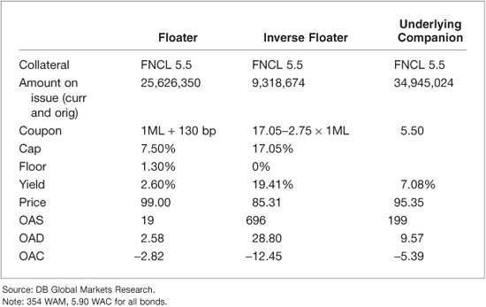
Floater
As well as the principal cash flows having different types, interest may also be paid in different ways. Most tranches have fixed-rate cash flows, as most collateral for CMOs has a fixed interest rate. However, it is possible to construct tranches with a floating rate of interest, generally tied to LIBOR, but conceptually to any market interest rate. One possibility is to use an interest rate swap to create a floating-rate bond. However, more likely is the division of a fixed-rate tranche into a “floater” and “inverse floater” whose interest rate moves down as the floater’s moves up (see Inverse Floater discussed later in the chapter).
Key components for a floater include:
• The index, such as LIBOR. Other indices used are constant maturity Treasury indices, such as 10Y CMT.
• The margin, or spread over the index paid to the investor.
• The cap, or maximum coupon rate that the floater can pay, inclusive of the margin paid over the index.
• The floor, or minimum coupon rate, often equal to the margin.
Example
Our example bond shown in Exhibit 26–12 is a companion floater. The average life is highly variable. The major issue for a bond buyer would be difficulty in hedging the risk of the embedded cap. Thus, higher cash-flow variability will in general push the OAS of a floater lower.
EXHIBIT 26–12
Example of a Floater
Analysis
Floating-rate bond analysis is similar to fixed-rate analysis in terms of examining cash flows and the bond’s OAS. However, the floater has the additional complexity of having embedded caps and floors to value (even if the floor is 0%). It is especially important to make sure the term structure model employed correctly values caps and floors at market values in this type of analysis. Additionally, an investor can price out an actual cap or floor for the expected average life of the security and see if the package of floater plus hedge makes sense.
Discount margin refers to the effective spread over the index once the bond’s price and a prepayment assumption are factored in. An investor would look at discount margin as well as OAS to determine value in a floater.
Note that a floater’s OAD (if uncapped) is effectively limited to the combination of index and index reset. Most of the duration of the floater duration would be due to the duration from the cap.
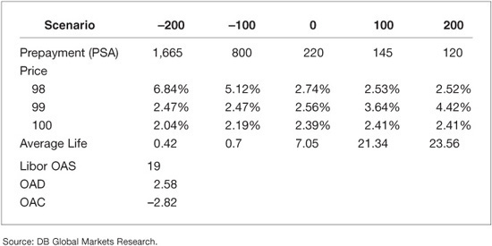
Inverse Floater
An inverse floater is typically created by dividing a fixed-rate tranche into a floating-rate portion and the inverse floater. The key understanding is that the sum of the parts (floater and inverse floater) must equal the whole (the underlying tranche) in terms of both interest and principal payments. (Also see the discussion later in the chapter dealing with “creation value.”)
Example
Our example is shown in Exhibit 26–13, a discount companion inverse floater. These bonds have a lot of duration and are often used as substitutes for POs. Our example has a highly variable average life, but high yields across interest rate scenarios.
EXHIBIT 26–13
Example of an Inverse Floater

Analysis
Inverse floater duration is increased by higher leverage in the inverse floater’s coupon formula. In our example bond, the underlying tranche has an OAD of 9.57 and the inverse floater’s leverage is 2.75. If the floater had a duration of 0, then the inverse floater’s OAD is roughly equivalent to 1 + leverage times the underlying tranche’s OAD. In this case, the floater has significant duration (over 2) because of the extension risk along with the relatively low coupon cap of the floater.
OAS analysis is important for analyzing inverse floaters, and as with floaters, inverse floaters have embedded caps and floors. Therefore, the term structure model is important for evaluation. Also, the prepayment model used to evaluate the inverse floater is critical. As market rates fall, the inverse floater’s coupon rises, but faster prepayments (and hence principal paydowns) may eat away the value of this to the bondholder. Effectively, the inverse floater buyer is leveraged to prepayments, and thus must be careful to examine the effect of variations in prepayment assumptions on bond valuation.
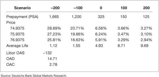
Inverse Floater versus Leveraged Collateral
Does OAS analysis work? One way to check is to compare inverse floaters with leveraged collateral positions. While at first glance it may appear that one should simply buy the bond with the highest OAS, in reality, the duration (or OAD) of the two assets being compared also matters significantly. To correctly compare inverse floaters with collateral, the collateral must be implicitly levered (by borrowing money) to the same duration as the inverse floater for the comparison to be fair. (The comparison is still not completely fair because leveraged collateral probably has more liquidity and easier funding than the inverse floater.)
In Exhibit 26–14, we can see that our prepayment model still prefers the inverse floater over a position of leveraged collateral. Levering the collateral involves investing a similar cash amount as for the inverse floater, then borrowing additional cash to buy more collateral until the investor has a similar duration and convexity exposure between the inverse floater and the leveraged collateral. In this example, we have borrowed money equivalent to the 2.75 times leverage of the inverse floater, assuming that we could borrow money at LIBOR flat.
EXHIBIT 26–14
Comparing Leveraged Collateral versus an Inverse Floater

Creation value is another method used to analyze inverse floaters. The value of floaters is relatively easy to determine, as they are relatively liquid and easy to price. Likewise, the underlying tranche for the floater/inverse combination is typically easy to price. Given those two prices, the arbitrage-free creation value of the inverse floater can be determined (Exhibit 26–15). Investors prefer to purchase inverse floaters at or below creation value in the secondary market.
EXHIBIT 26–15
Floater + Inverse Floater = Underlying Companion Bond
Trade against Forward Rates
Some investors buy inverse floaters as a trade against forward rates rising as fast as the market would suggest. For example, the yield of our inverse floater at unchanged rates and 220 PSA is 19.41%. The yield assuming this prepayment speed but forward rates is 18.4%. If rates rise more slowly than forward rates suggest, the true yield of the bond will be somewhere in between the two numbers.
Analyzing inverse floaters is complex and can be done in many different ways. They are not as liquid as regular tranches. The reward may be discovering some true value in the bonds, or taking advantage of specific views on the market.
Interest-Only and Principal-Only Tranches
Interest-only tranches (IOs) come in several forms. The primary one we will discuss is “trust IOs,” in which collateral is contributed to an IO/PO deal by dealers, a small fee is charged by a GSE or Agency, and IO and PO tranches are returned to the dealers involved in proportion to their collateral contribution. This type of structure gets its own IO/PO trust number, hence the name. An IO can also be created by stripping interest off a CMO tranche or in other ways, which typically result in CMO tranches with IO characteristics. Trust IOs tend to have the most liquidity, as they are large size deals that trade on broker screens, while smaller deals have less price transparency.
IOs typically have negative duration. If interest rates rise, prepayment speeds tend to slow. Slower speeds benefit the IO holder, who wants the collateral factor to stay as high for as long as possible. Once loans prepay, they stop paying interest beyond the month in which prepayment occurs. An IO investor wants prepayments to be as slow as possible. In the most extremely negative case, an investor could buy an IO and discover the entire tranche has paid off in that month, reported in the following month.
The principal only (PO) is the complement of the IO. It returns only the principal portion of the pass-through. Thus, a PO holder would prefer prepayments to be extremely fast. Under a dollar price of approximately $85-00 (which is typical), POs have positive convexity. This makes them useful for hedging purposes, for example hedging mortgage servicing rights.
Example
Exhibit 26–16 shows an example of an IO. Since trust IO and PO pricing is relatively liquid, most of the analysis for IOs and POs will concern an investor’s view of prepayments or interest rates versus the market’s (as represented by IO/PO pricing). Nevertheless, IO/PO prices can also fluctuate due to technicals, including short squeezes on certain tranches. Note how the IO in Exhibit 26–16 has a high negative OAD.

Exhibit 26–17 shows an example PO from the same Trust deal. Some investors buy POs for prepayment protection or positive convexity, but others buy them simply to add duration to their mortgage portfolio. As interest rates drop, observe that the PO yield rises significantly due to increased prepayments. Often, as in our hypothetical example, the PO will have a negative OAS in return for its positive convexity. Effectively, an investor is paying a premium to buy call options when they buy a PO.
Analysis
IO/PO analysis using OAS models or other techniques is notoriously complex, and even seasoned traders have lost money due to technicals in the IO market. As IOs and POs are notoriously sensitive to even small changes in prepayment assumptions, one must be very careful to examine the model used to calculate OASs. Variables such as seasoning and burnout are magnified many times in between analyzing the collateral and the IO/PO derivative.
Creation value can also be used to analyze IOs and POs, similar to the analysis of inverse floater/floater combinations. For Trust IOs and POs, at first the combination (combo) typically trades at a small premium above collateral. The combination cannot trade significantly below the price of collateral, because they may be recombined into collateral for a small fee and sold. However, the combination may trade at a price significantly above TBA collateral for a number of reasons:
• The underlying collateral is valuable, for example it has seasoning worth a pay-up to TBA collateral.
• There is a squeeze or scarcity of the IO or PO, which raises the price of the combination in turn. Sometimes POs get restructured in other deals, potentially leaving them dear.
Historical analysis of IO and PO OAS numbers may be somewhat useful, but ends up being highly prepayment and OAS model dependent.
Premium tranche/IO arbitrage is another way to compare relative value of IOs versus regular classes of CMOs. For example, a PAC IO plus a stripped down PAC should equal the value of the full coupon PAC, or there is an arbitrage. This is similar to the recombination value of an inverse floater. In practice, since many investors are willing to accept tighter spreads for lower dollar price PAC bonds, we can see arbitrage opportunities occur during deal pricings which make the restructuring of a premium PAC tranche into a stripped-down coupon PAC and a PAC IO attractive.
For POs, some investors may be using them to hedge other assets, such as mortgage servicing rights (MSR). In that case, all the above analysis may be performed, but the investor probably also wants to check how well correlated changes in price of the PO will match changes in price of the hedged asset.
Unusual Features
Note that IOs can be stripped off of any CMO type, for example PACs, creating PAC IOs. This class of bond will behave like a high yielding PAC within the band, but if prepayments speed up, will pay off quickly, perhaps leaving a loss for the investor. Other non-Trust IOs must be examined carefully as to the nature of their cash flows.
Exotics
We now describe a number of exotic CMOs for the sake of completeness, but will not spend a lot of time looking at individual bonds.
Inverse IOs
Inverse IOs are created by stripping the premium portion off an inverse floater. In some respects they behave as an interest rate floor. At times, their pricing has been described in relation to floor prices (e.g., 80%). However, they are more like “knockout” floors because if interest rates fall enough, prepayment rates will speed up and pay down the notional principal of the tranche, reducing the remainder of the investment to zero. Because of their illiquidity, these bonds are difficult to hedge and value even more so than trust IOs.
Inverse IOs are highly levered to one’s interest rate scenario and prepayment forecast. It is important to analyze how small variations in prepayment or interest rate assumptions change the potential value of the bond.
Jump Zs
A jump Z reacts to fast prepayments by suddenly shifting from accrual to paying interest and principal (becoming a “payer”). This option can be of great value to the investor if the Z-bond is at a discount price. Note also that some Jump Zs are sticky, meaning once the “payer” trigger has been pulled, they continue to pay even if prepayment rates subsequently drop.
Structured POs
POs themselves can be structured into TAC POs, Super POs (companion POs), etc. Analysis is similar to that for PO analysis, except the bonds will probably be even more sensitive to slight changes in prepayment assumptions.
AGENCY VERSUS NONAGENCY CMOs
While most investors who can buy agency pass-throughs are allowed to buy agency CMOs, certain investors cannot participate in the nonagency CMO market. Here, we describe some of the differences between the two markets (see Exhibit 26–18 for a synopsis). Nonagency CMOs are discussed in more detail in Chapter 31.
EXHIBIT 26–18
Agency versus Nonagency CMO Differences

AGENCY CMO ANALYSIS
The following section looks at how investors analyze and use agency CMOs. We also cover term structure and prepayment models briefly.
Analysis for Regular CMO Tranches
CMO analysis depends upon investor needs. While relative value may seem to be one answer, one rule does not necessarily hold for all investors. The definition of relative value can be different for different investors. Other investors have portfolio constraints. For example, an insurance company may need assets that closely match liabilities even if interest rates exhibit large moves.
Investor Goals and Constraints
Investors can have many goals and constraints when purchasing CMOs. For example:
• Insurance companies and banks sometimes have yield levels (bogies) below which they do not wish to purchase bonds.
• Relative value investors may require a certain OAS, or OAS advantage versus collateral.
• Hedge funds may require a certain amount of liquidity in purchases they make, both for bonds and potential hedges (such as cancelable swaps). If liquidity in the bond or the hedges is insufficient, they may decline to do an otherwise attractive trade.
• Funded investors may need to issue debt or raise equity before adding MBS. If the environment is not amenable to such issuance, then CMO purchases may be delayed.
• Banks may have internal maturity or duration restrictions or preferences on bonds for their portfolio.
• Individual or institutional investors may have a top dollar price limit above which they will not purchase bonds.
Perhaps the variability of investors explains why there are so many different kinds of CMOs, some unique. Different requirements and views are what makes a market.
Cash-Flow Analysis
For most regular tranche types, cash-flow analysis consists of testing various prepayment models and static prepayments to determine what the sensitivity of a bond is to changes in interest rates. This analysis would include a comparison of the negative convexity of different CMO bonds.
For some investors, cash-flow analysis becomes more detailed, as they may be trying to hedge their own stream of liabilities, or perhaps they are hedging the CMO with an amortizing swap.
Finally, for nonstandard tranches, it pays to examine the cash-flow waterfall and test various interest-rate scenarios, examining the results in terms of cashflow streams. It is important to check for bonds that have unusual cash flows. For example, anything that could cause a bond to have a longer-than-expected maturity, or a gap when principal was not paid would be suspect.
OAS Analysis
For most regular CMO tranches, OAS analysis is relatively useful. For similar tranches off similar collateral, it is easy to use OAS to determine relative value of bonds. In addition, comparing OAS numbers for CMOs versus underlying collateral also is straightforward. The more difficult issue is how to compare OAS numbers of tranches of different durations. For example, often longer dated tranches are at higher OAS numbers than similar shorter dated tranches. This structural issue makes it difficult to evaluate relative value of longer versus shorter dated CMOs.
More issues in OAS analysis are presented later in this chapter and in Chapter 41.
Hedging
For normal CMO tranches, OADs are an acceptable way to calculate how to hedge. However, wide window sequentials may require hedging on multiple points on the yield-curve to avoid yield-curve risk, similar to hedging yield-curve risk in the underlying collateral. Exhibit 26–19 shows how the bulk of duration risk may be in the 10-year area for a specific bond, but hedging in the 2 year, 5 year, and 30 year would help reduce yield-curve risk.
EXHIBIT 26–19
Partial Durations of a Five-Year-Wide Window Sequential

Issues in OAS Analysis
There are a number of issues in OAS analysis to discuss in order to determine if the OAS received on a bond is truly what the investor seeks to find out: the spread of the mortgage backed security, ex-option cost, versus a benchmark such as swaps. While in the 1980s and early 1990s, the primary variable differentiating OAS numbers was the prepayment model, at this point in the technology, the term structure model has become equally as important. We cover a number of other issues in this section, such as deal call risk, and variations among prepayment models.
Term Structure Model
As mortgages have linked more tightly over time with the OTC derivatives markets (swaps and swaptions), modeling the relationship between these two markets has become critical. When swaps and swaptions are used to hedge MBS (or vice versa), the two markets need to be evaluated using the same term-structure model and the same assumptions, or else different, and perhaps erroneous, results can be obtained.
While a one-factor interest-rate model was used in the past and may work reasonably for pass-throughs, it is clearly not enough if an investor is looking at ARMs, floaters, or inverse floaters of any kind. More degrees of freedom for modeling the yield-curve are needed. Therefore, in order to keep analysis consistent among different types of MBS tranches and derivatives, it appears critical to use the least common denominator of term structure models that will accommodate all possible tranche types and analysis, and not succumb to using different models for different types of bonds or situations.
Advances in term structure modeling have placed the following features into the hands of mortgage analysts:
• Multiple knots on the yield-curve.
• Correct pricing of OTC derivatives using the model.
• Pricing in a volatility “skew” (i.e., options not struck at-the-money may be priced at a different volatility than standard at-the-money options).
• Sophisticated simulation of future mortgage interest rates based on the swaps curve and volatility.
The point is that a term structure model that does not do these things opens up arbitrage opportunities against an investor using it. In an extreme case, flaws in the term structure model will misstate value and risk numbers associated with a CMO.
Forward Curve Bias
Despite all the care being put into term structure models, and their freedom from arbitrage, it is important also for investors to recognize the forward curve bias in these models, which creates a paradox.
• In order to remain arbitrage free, the term structure model must use the forward yield-curve as its base case.
• In practice, the forward yield-curve is usually wrong.
How can we reconcile these two facts?
The short answer is that we should use the forward yield-curve, because if we do not believe something that it is predicting, we can trade against it and make money if we are correct. At times, the second point becomes plainly obvious. For example, when the yield-curve is extremely steep, forward rates predict massive flattening of the yield-curve over a short period of time. If the Fed appears to be on hold during this time, are we likely to get the full amount of the yield-curve flattening? Probably not. However, it may be easier to trade on this view directly in the derivatives or futures market rather than trying to implement it in the mortgage market.
Prepayment Model
The prepayment model is a very important component of mortgage analysis and OAS. Over time, prepayments have become more efficient. While most prepayment models address the standard issues of age, relative coupon, etc., there are now various subtleties for which a model needs to account:
• Does the model account for “credit impaired” mortgages issued at above market rates?
• How does prepayment “burnout” work in the model? Can burnout be erased over time?
• Does the model account for “underwater” mortgages correctly (where the loan is for more than the home is worth)?
A prepayment model that is out of date or incorrect, even if only on a small segment of the market (e.g., high-premium mortgages) can have a large impact on an OAS because OAS models tend to generate some paths with very high and low interest rates—testing the boundaries of prepayment models and their ability to generate reasonable prepayment forecasts at out-of-sample interest rates.
Why A + B Can Be Greater Than C…
One of the last topics we will cover in this section is why A + B > C, even if A and B are made up of the component cash flows of C. Here are some factors.
• A and B are unique and more cannot be created. For example, once a Trust IO/PO deal is closed, additional collateral cannot be added later to increase the size of the deal. Thereafter, a squeeze in A or B will increase their price in relation to C, which is simply TBA collateral. A + B can never be less than (C – transaction cost) for long, as this would create a recombination arbitrage.3
• A or B is getting squeezed. One of the risks in the IO/PO market is that bonds can be re-securitized and hence lost to the possibility of recombination. For example, if virtually all of the POs in a Trust deal are re-securitized, the remaining POs will be in very high demand to hedge the remaining IO tranches. In addition, trust IO/PO sizes can be small enough that one dealer or investor can potentially squeeze the market in one of these bonds, making A + B > C.
• The underlying collateral is valuable. Sometimes A + B may be compared with the wrong C. For example, comparing a Trust IO and PO to TBA collateral may be appropriate most of the time. However, after the deal is seasoned for a while, the underlying collateral itself may be worth a pay-up to TBAs (seasoned collateral typically commands a premium price to TBAs).
Examining Deal Call Risk
A feature in many CMO deals, but not discussed often and sometimes not modeled, is the embedded call. Calls were originally conceived as a way to limit ongoing fixed expenses for deal trustees on CMOs that have shrunk to a very small size, but the implications for investors can be significant. For example, the last cash-flow holder will typically be exposed to the call. A call that sounds small for an entire deal (say, 1%), may actually make up a large portion of the last tranche remaining in a CMO deal. For a tranche that was only 5% of the deal’s original principal, a 1% cleanup call is exercised when 20% of the last tranche is remaining. The impact for investors of other tranches is de minimus, but obviously can be large for the last cash-flow holder.
The good news is this call is exercised most of the time, because the fixed costs of the deal tend to be large enough that the trustee wants to exercise the call whenever possible. This assumption makes analysis easy. However, if the price of the collateral is significantly below par, calling the deal costs the trustee money. Analysis of the probability of call of deals in this situation is difficult. Therefore, the bond holder may want to run the bond with and without the call to assess the possible impact.
Investor Types and Behavior
In this section, we examine different types of investors, such as commercial banks. We cover the following information for each:
• Types of CMOs typically purchased by these institutions
• Methods potentially used by these institutions for bond selection
Historically, banks have been the largest holders of MBS.
Banks
Banks are large consumers of the CMO product. For many banks, the longer duration and possible duration extension of pass-throughs does not match their liabilities adequately. Often, it is easier for many banks to achieve a shorter duration security or less extension risk by buying appropriately structured CMO bonds than pass-throughs. Banks are typically buy and hold investors in CMOs, although some bonds may be placed in the trading account.
In general, banks focus on shorter duration CMOs. A 10-year bond typically does not fit the liability structure of a bank. A two-year sequential CMO is a typical purchase for a bank. In general, banks will accept some prepayment and convexity risk in order to get a better spread. Therefore, banks tend to prefer sequentials over PAC bonds. Banks do very little hedging of their negative convexity using the options market, although they may delta hedge their mortgage position as its duration changes.
CMO selection at banks generally comes down to a few things: yield bogey, duration, and OAS. In general, a bank will have a target net interest margin over their cost of funds in order to purchase a security. This target may be translated into a yield or spread bogey over a market rate. Also, a bank may not want to take too much duration risk, so the duration of the security must fit the asset-liability framework of the bank, or it must be prepared to hedge the duration of the CMO. Some banks use OAS to determine relative value among tranches, but in general asset-liability and liquidity concerns tend to dominate their CMO purchase decisions.
Note also that banks are the largest consumer of mortgage “whole loans,” or mortgages that are not securitized. These whole loans are mostly ineligible for agency securitization, or are ARMs or hybrid ARMs.
Insurance Companies
Insurance companies buy CMOs across the spectrum of “regular” tranches—PACs, sequentials, and PACquentials. Property and casualty companies tend to buy shorter maturity tranches, such as two year sequentials. Life insurance companies are looking for more structure to match against their liabilities and are more likely to purchase longer duration bonds, such as 10-year PACs. While MBS are a break from the credit risk that insurance companies typically take on the corporate bonds in their investment portfolio, they are well aware of the convexity risk that they are taking in MBS. In 1995, S&P devised a “convexity test” that penalized insurance companies for having negative convexity in their portfolios. This served primarily to reduce mortgage holdings at some particularly large “outlier” firms that held lots of MBS, but has also generally reduced MBS holdings over time to smaller amounts at insurance companies.
In general, insurance companies may have restrictions on selling CMOs because of gain or loss constraints. Property and casualty companies may sell bonds against claims (e.g., after a hurricane).
Money Managers
Money managers vary in sophistication. They generally are not subject to gain/loss constraints because they mark-to-market constantly, unless they are managing a separate account for a financial institution. Some money managers are active in the CMO derivatives market, but many are not. Most money managers are benchmarked against an index that contains pass-throughs. Therefore, any CMO is effectively an “out of index” bet for them. They will typically be comparing that CMO either to collateral or perhaps to Treasuries/agencies for certain types of CMOs. OAS analysis tends to be an important tool for them.
Liquidity tends to be a bigger issuer for money managers than for insurance companies. The money manager may need to be able to shift assets around quickly, and thus is prepared to give up something in order to have better liquidity. Most money managers own many more pass-throughs than CMOs because of this fact. In addition, pass-throughs have the opportunity to finance special (via the dollar roll market). Income from special financing can be a windfall for money managers, as this income is typically not included in mortgage index returns the money managers are benchmarked against.
Money managers frequently take long-term views about strategy in mortgages. One type of view is to have a portfolio that has better (or worse) convexity than their benchmark index. A money manager can typically get better convexity by buying PAC bonds, or give up convexity to gain yield by buying companion bonds or certain types of sequentials or broken PACs.
Pension Funds
Pension funds in some ways operate similarly to money managers. However, ERISA (pension fund law) or investor considerations sometimes keep them from investing in mortgage derivatives. Similar to life insurance companies, they can be interested in longer duration tranches at times.
Hedge Funds
Hedge funds can operate in a manner similar to money managers, but at times they enter into more complex trades involving OTC derivatives. For example, they might buy a CMO and try to hedge its cash flows over time using swaps and options, netting a positive spread that they hope to earn over time.
Certain hedge funds specialize in mortgage derivatives: inverse floaters, IOs, POs, inverse IOs, etc. They use sophisticated models to value these tranches, purchase them, and hedge them. One of the main issues for these funds will be pricing of their inventory (as individual bonds may not trade for months) and liquidity.
Retail Investors/Regional Dealers
Many CMOs, including CMO derivatives such as inverse floaters, end up in the hands of regional dealers. In turn, these regional dealers may sell those bonds to retail clients. In general, yield tends to be the focus of these buyers, and thus companion bonds are often sold via this channel.
Note that any broker who sells CMOs to retail investors must include a series of special disclaimers that is mandated by securities regulation.
Lessons from the Past
Investors in MBS, and especially in derivative MBS, have gone out of business in the past. In a crisis, while the mortgage market may continue to trade via pass-throughs, the CMO market can lose liquidity, and the derivatives market can practically stop trading for some period of time. Investors should be prepared for all risks, including the risk of illiquidity and radical changes in pricing due to such illiquidity. Dealers must make sure they “know their customer” and that the customer is buying bonds appropriate for their goals.
KEY POINTS
• Agency CMOs are structured by broker-dealers into multiple tranches using agency pass-throughs as collateral. The deals are wrapped and issued by Fannie Mae, Freddie Mac, or Ginnie Mae. Ginnie Mae has the full faith and credit backing of the U.S. government, while the other two have an implied guarantee.
• Agency CMOs can be a safe, attractive investment for banks, mutual funds, insurance companies, and other institutional investors. Standard types of CMO tranches include PACs (created to mimic corporate bonds), sequentials (that time tranche principal cash flows), and companions (that return a high yield in return for highly variable principal cash flows).
• Unlike most other bonds, all MBS (including CMOs) have unpredictable return of principal, creating the opportunity of higher yield and the risk of callability. The homeowner in the United States typically has the option to refinance at any time, effectively exercising a call to the investor. Using OAS and prepayment models helps investors understand the nature of the MBS they own or are buying.
• Analysis of CMOs depends to some degree on the type of investor: yield tables and OAS analysis are the most popular. Banks typically look at average life profiles, yield tables, and may consider OAS. Money managers tend to be more focused on OAS and less on yield.
• CMO derivatives can provide hedging benefits or unusual return profiles. For example, Interest-only strips have a negative duration—they generally increase in price as interest rates rise. Inverse floaters have bond coupons that rise as interest rates fall, sometimes creating bonds with very long OADs.