CHAPTER
THIRTY-SIX
OVERVIEW OF FORWARD RATE ANALYSIS

ANTTI ILMANEN, PH.D.

Managing Director
AQR Capital Management (Europe) LLP

Over the years, advances have been made in both the theoretical and the empirical analysis of the term structure of interest rates. However, such analysis is often very quantitative, and it rarely emphasizes practical investment applications. In this chapter we briefly describe the computation of par, spot, and forward rates, present a framework for interpreting the forward rates by identifying their main determinants, and develop practical tools for using the information in forward rates in active bond portfolio management.

The three main influences on the Treasury yield-curve shape are (1) the market’s expectations of future rate changes, (2) bond risk premiums (expected return differentials across bonds of different maturities), and (3) convexity bias. Conceptually, it is easy to divide the yield-curve (or the term structure of forward rates) into these three components. It is much harder to interpret real-world yield-curve shapes, but the potential benefits are substantial. For example, investors often wonder whether the curve steepness reflects the market’s expectations of rising rates or a positive risk premium. The answer to this question determines whether a duration extension increases expected returns. It also shows whether we can view forward rates as the market’s expectations of future spot rates. In addition, in this chapter we will explain how the market’s curve reshaping and volatility expectations influence the shape of today’s yield-curve. These expectations determine the cost of enhancing portfolio convexity via a duration-neutral yield-curve trade.¹

Forward rate analysis also can be valuable in direct applications. Forward rates may be used as break-even rates to which subjective rate forecasts are compared or as relative-value tools to identify attractive yield-curve sectors.²

COMPUTATION OF PAR, SPOT, AND FORWARD RATES

At the outset, it is useful to review the concepts yield-to-maturity, par yield, spot rate, and forward rate to ensure that we are using our terms consistently. Appendix 36A is a reference that describes the notation and definitions of the main concepts used in this chapter. Our analysis focuses on government bonds that have known cash-flows (no default risk, no embedded options). Yield-to-maturity is the single discount rate that equates the present value of a bond’s cash-flows to its market price. A yield-curve is a graph of bond yields against their maturities. (Alternatively, bond yields may be plotted against their durations, as we do in many of the exhibits presented in this chapter.) The best-known yield-curves are the on-the-run Treasury curve and the interest-rate-swap curve. On-the-run bonds are the most recently issued government bonds at each maturity sector. Since these bonds are always issued with price near par (100), the on-the-run curve often resembles the par yield-curve, which is a curve constructed for theoretical bonds whose prices equal par. The swap curve based on receive-fixed, pay-floating contracts is by construction a par curve.

While the yield-to-maturity is a convenient summary measure of a bond’s expected return—and therefore a popular tool in relative-value analysis—the use of a single rate to discount multiple cash-flows can be problematic unless the yield-curve is flat. First, all cash-flows of a given bond are discounted at the same rate, even if the yield-curve slope suggests that different discount rates are appropriate for different cash-flow dates. Second, the assumed reinvestment rate of a cash-flow paid on a given date can vary across bonds because it depends on the yield of the bond to which the cash-flow is attached. In this chapter we will show how to analyze the yield-curve using simpler building blocks—single cash-flows and one-period discount rates—than the yield-to-maturity, an average discount rate of multiple cash-flows with various maturities.

A coupon bond can be viewed as a bundle of zero-coupon bonds (zeros). It can be unbundled to a set of zeros that can be valued separately. Then these can be bundled back together into a more complex bond whose price should equal the sum of the component prices.³ The spot rate is the discount rate of a single future cash-flow such as a zero. Equation (36.1) shows the simple relation between an n-year zero’s price P_n and the annualized n-year spot rate s_n.

A single cash-flow is easy to analyze, but its discount rate can be unbundled even further to one-period rates. A multiyear spot rate can be decomposed into a product of one-year forward rates, the simplest building blocks in a term structure of interest rates. A given term structure of spot rates implies a specific term structure of forward rates. For example, if the m-year and n-year spot rates are known, the annualized forward rate between maturities m and n, that is, f_m,n, is easily computed from Eq. (36.2).

The forward rate is the interest rate for a loan between any two dates in the future, contracted today. Any forward rate can be “locked in” today by buying one unit of the n-year zero at price P_n 100/(1 + s_n)ⁿ and by shortselling P_n/P_m units of the m-year zero at price P_m = 100/(1 + s_m)^m. (Such a weighting requires no net investment today because both the cash inflow and cash outflow amount to P_n.) The one-year forward rate (f_n−1,n such as f_1,2, f_2,3, f_3,4, . . .) represents a special case of Eq. (36.3) where m = n − 1. The spot rate represents another special case where m = 0; thus s_n = f_0,n.

To summarize, a par rate is used to discount a set of cash-flows (those of a par bond) to today, a spot rate is used to discount a single future cash-flow to today, and a forward rate is used to discount a single future cash-flow to another (nearer) future date. The par yield-curve, the spot-rate curve, and the forward-rate curve contain the same information about today’s term structure of interest rates.⁴ If one set of rates is known, it is easy to compute the other sets.⁵ Exhibit 36–1 shows a hypothetical example of the three curves. In Appendix 36B, we show how the spot and forward rates were computed based on the par yields.

EXHIBIT 36–1
Par, Spot, and One-Year Forward Rate Curves

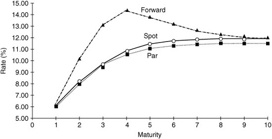
In this example, the par and spot curves are monotonically upward-sloping, whereas the forward rate curve⁶ is first upward-sloping and then inverts (because of the flattening of the spot curve). The spot curve lies above the par curve, and the forward rate curve lies above the spot curve. This is always the case if the spot curve is upward-sloping. If it is inverted, the ordering is reversed: The par curve is highest, and the forward curve lowest. Thus loose characterizations of one curve (e.g., steeply upward-sloping, flat, inverted, humped) generally are applicable to the other curves. However, the three curves are identical only if they are horizontal. The forward rate curve magnifies any variation in the slope of the spot curve. One-year forward rates measure the marginal reward for lengthening the maturity of the investment by one year, whereas the spot rates measure an investment’s average reward from today to maturity n. Therefore, spot rates are (geometric) averages of one or more forward rates. Similarly, par rates are averages of one or more spot rates; thus par curves have the flattest shape of the three curves. In Appendix 36C, we discuss further the relation between spot and forward rate curves.

It is useful to view forward rates as break-even rates. The implied spot rates one year forward (f_1,2, f_1,3, f_1,4, . . .) are, by construction, equal to such future spot rates that would make all government bonds earn the same return over the next year as the (riskless) one-year zero. For example, the holding-period return of today’s two-year zero (whose rate today is s₂) will depend on its selling rate (as a one-year zero) in one year’s time. The implied one-year spot rate one year forward (f_1,2) is computed as the selling rate that would make the two-year zero’s return [the left-hand side of Eq. (36.3)] equal to the one-year spot rate [the right-hand side of Eq. (36.3)]. Formally, Eq. (36.3) is derived from Eq. (36.2) by setting m = 1 and n = 2 and rearranging.

Consider an example using numbers from Exhibit 36B–1 in Appendix 36B, where the one-year spot rate (s₁) equals 6% and the two-year spot rate (s₂) equals 8.08%. Plugging these spot rates into Eq. (36.3), we find that the implied one-year spot rate one year forward (f_1,2) equals 10.20%. If this implied forward rate is exactly realized one year hence, today’s two-year zero will be worth 100/1.1020 = 90.74 next year. Today, this zero is worth 100/1.0808² = 85.61; thus its return over the next year would be 90.74/85.61 − 1 = 6%, exactly the same as today’s one-year spot rate. Thus 10.20% is the break-even level of the future one-year spot rate. In other words, the one-year rate has to increase by more than 420 basis points (10.20% − 6.00%) before the two-year zero underperforms the one-year zero over the next year. If the one-year rate increases, but by less than 420 basis points, the capital loss of the two-year zero will not fully offset its initial yield advantage over the one-year zero.

More generally, if the yield changes implied by the forward rates are realized subsequently, all government bonds, regardless of maturity, earn the same holding-period return. In addition, all self-financed positions of government bonds (such as long a barbell versus short a bullet) earn zero return; that is, they break even. However, if the yield-curve remains unchanged over a year, each n-year zero earns the corresponding one-year forward rate f_n−1,n. This can be seen from Eq. (36.2) when m = n − 1; 1 + f_n−1,n equals (1 + s_n)ⁿ/(1 + s_n−1)ⁿ⁻¹, which is the holding-period return from buying an n-year zero at rate s_n and selling it one year later at rate s_n−₁. Thus the one-year forward rate equals a zero’s horizon return for an unchanged yield-curve. See Appendix 36C for details.

MAIN INFLUENCES ON THE YIELD-CURVE SHAPE

In this section we describe some economic forces that influence the term structure of forward rates or, more generally, the yield-curve shape. The three main influences are the market’s rate expectations, the bond risk premiums (expected return differentials across bonds), and the so-called convexity bias. In fact, these three components fully determine the yield-curve; it can be shown that the difference between each one-year forward rate and the one-year spot rate is approximately equal to the sum of an expected spot-rate change, a bond risk premium, and the convexity bias.⁷ We first discuss separately how each component alone influences the curve shape and then analyze their combined impact.

Expectations

It is clear that the market’s expectations of future rate changes are one important determinant of the yield-curve shape. For example, a steeply upward-sloping curve may indicate market expectations of near-term Fed tightening or of rising inflation. However, it may be too restrictive to assume that the yield differences across bonds with different maturities only reflect the market’s rate expectations. The well-known pure expectations hypothesis has such an extreme implication. The pure expectations hypothesis asserts that all government bonds have the same near-term expected return (as the nominally riskless short-term bond) because the return-seeking activity of risk-neutral traders removes all expected return differentials across bonds. Near-term expected returns are equalized if all bonds that have higher yields than the short-term rate are expected to suffer capital losses that offset their yield advantage. When the market expects an increase in bond yields, the current term structure becomes upward-sloping so that any long-term bond’s yield advantage and expected capital loss (owing to the expected yield increase) exactly offset each other. Stated differently, if investors expect that their long-term bond investments will lose value owing to an increase in interest rates, they will require a higher initial yield as a compensation for duration extension. Conversely, expectations of yield declines and capital gains will lower current long-term bond yields below the short-term rate, making the term structure inverted.

The same logic—that positive (negative) initial yield spreads offset expected capital losses (gains) to equate near-term expected returns—also holds for combinations of bonds, including duration-neutral yield-curve positions. One example is a trade that benefits from the flattening of the yield-curve between two- and ten-year maturities: selling a unit of the two-year bond, buying a duration-weighted amount (market value) of the ten-year bond, and putting the remaining proceeds from the sale to “cash” (very short-term bonds). Given the typical concave yield-curve shape, such a curve-flattening position earns a negative carry.⁸ The trade will be profitable only if the curve flattens enough to offset the impact of the negative carry. Implied forward rates indicate how much flattening (narrowing of the two- to ten-year spread) is needed for the trade to break even.

In the same way as the market’s expectations regarding the future level of rates influence the steepness of today’s yield-curve, the market’s expectations regarding the future steepness of the yield-curve influence the curvature of today’s yield-curve. If the market expects more curve flattening, the negative carry of the flattening trades needs to be larger (to offset the expected capital gains), which makes today’s yield-curve more concave (curved). Exhibit 36–2 illustrates these points. This figure plots coupon bonds’ yields against their durations or, equivalently, zeros’ yields against their maturities, given various rate expectations. Ignoring the bond risk premium and convexity bias, if the market expects no change in the level or slope of the curve, today’s yield-curve will be horizontal. If the market expects a parallel rise in rates over the next year (but no reshaping), today’s yield-curve will be linearly increasing (as a function of duration). If the market expects rising rates and a flattening curve, today’s yield-curve will be increasing and concave (as a function of duration).⁹

EXHIBIT 36–2
Yield Curves Given the Market’s Various Rate Expectations

Bond Risk Premium

A key assumption in the pure expectations hypothesis is that all government bonds, regardless of maturity, have the same expected return. In contrast, many theories and empirical evidence suggest that expected returns vary across bonds. We define the bond risk premium as a longer-term bond’s expected one-period return in excess of the one-period bond’s riskless return. A positive bond risk premium would tend to make the yield-curve slope upward. Various theories disagree about the sign (+/−), the determinants, and the constancy (over time) of the bond risk premium. The classic liquidity premium hypothesis argues that most investors dislike short-term fluctuations in asset prices; these investors will hold long-term bonds only if they offer a positive risk premium as a compensation for their greater return volatility. Also, some modern asset-pricing theories suggest that the bond risk premium should increase with a bond’s duration, its return volatility, or its covariance with market wealth. In contrast, the preferred-habitat hypothesis argues that the risk premium may decrease with duration; long-duration liability holders may perceive the long-term bond as the riskless asset and require higher expected returns for holding short-term assets. While academic analysis focuses on risk-related premiums, market practitioners often emphasize other factors that cause expected return differentials across the yield-curve. These include liquidity differences between market sectors, institutional restrictions, and supply and demand effects. We use the term bond risk premium broadly to encompass all expected return differentials across bonds, including those caused by factors unrelated to risk.

Historical data on U.S. Treasury bonds provide evidence about the empirical behavior of the bond risk premium. For example, the fact that the Treasury yield-curve has been upward-sloping more than 90% of the time in recent decades may reflect the impact of positive bond risk premiums. Historical average returns provide more direct evidence about expected returns across maturities than do historical yields. Even though weekly and monthly fluctuations in bond returns are mostly unexpected, the impact of unexpected yield rises and declines should wash out over a long sample period. Therefore, the historical average returns of various maturity sectors over a relatively trendless sample period should reflect the long-run expected returns.

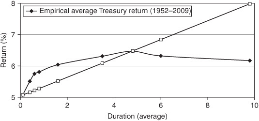
Exhibit 36–3 shows the empirical average return curve as a function of average duration and contrasts it with a popular theoretical expected return curve, one that increases linearly with duration. The theoretical bond risk premiums are measured in the exhibit by the difference between the annualized expected returns at various duration points and the annualized return of the riskless one-month bill (the leftmost point on the curve). Similarly, the empirical bond risk premiums are measured by the historical average bond returns (at various durations) in excess of the one-month bill.¹⁰ Historical experience suggests that the bond risk premiums are not linear in duration but that they increase steeply with duration in the front end of the curve and much more slowly after two years. The concave shape may reflect the demand for long-term bonds from pension funds and other long-duration liability holders.

Exhibit 36–3 may give us the best empirical estimates of the long-run average bond risk premiums at various durations. However, empirical studies also suggest that the bond risk premiums are not constant but vary over time. That is, it is possible to identify in advance periods when the near-term bond risk premiums are abnormally high or low. These premiums tend to be high after poor economic conditions when the yield-curve is steep, amid high inflation expectations and related inflation uncertainty. These premiums tend to be lower and even turn negative when Treasury prices benefit from safe-haven premiums (amid equity market weakness and negative stock-bond correlation, as in 1998 and 2002) or from scarcity premiums (amid fiscal surpluses and expectations of dwindling government bond markets, as in 2000).¹¹

EXHIBIT 36–3
Theoretical and Empirical Bond Risk Premiums

Convexity Bias

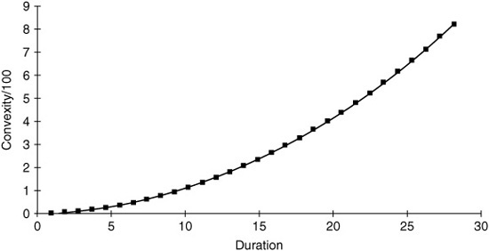
The third influence on the yield-curve—convexity bias—is probably the least well known. Different bonds have different convexity characteristics, and the convexity differences across maturities can give rise to (offsetting) yield differences. In particular, long-term bonds exhibit very high convexity (see panel a of Exhibit 36–4), which tends to depress their yields. Convexity bias refers to the impact these convexity differences have on the yield-curve shape.

Convexity is closely related to the nonlinearity in the bond price-yield relationship. All noncallable bonds exhibit positive convexity; their prices rise more for a given yield decline than they fall for a similar yield increase. All else being equal, positive convexity is a desirable characteristic because it increases bond return (relative to return in the absence of convexity) whether yields go up or down—as long as they move somewhere. Because positive convexity can only improve a bond’s performance (for a given yield), more convex bonds tend to have lower yields than less convex bonds with the same duration.¹² In other words, investors tend to demand less yield if they have the prospect of improving their returns as a result of convexity. Investors are primarily interested in expected returns, and these high-convexity bonds can offer a given expected return at a lower yield level.

EXHIBIT 36–4 (a)
Illustration of Convexity Bias

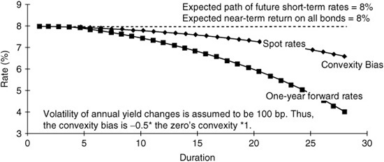
Panel b of Exhibit 36–4 illustrates the pure impact of convexity on the curve shape by plotting the spot-rate curve and the curve of one-year forward rates when all bonds have the same expected return (8%) and the short-term rates are expected to remain at the current level. With no bond risk premiums and no expected rate changes, one might expect these curves to be horizontal at 8%. Instead, they slope down at an increasing pace because lower yields are needed to offset the convexity advantage of longer-duration bonds and thereby to equate the near-term expected returns across bonds.¹³ Short-term bonds have little convexity, so there is little convexity bias at the front end of the yield-curve, but convexity can have a dramatic impact on the curve shape at very long durations. Convexity bias can be one of the main reasons for the typical concave yield-curve shape (i.e., for the tendency of the curve to flatten or invert at long durations).

EXHIBIT 36–4 (b)
Pure Impact of Convexity on the Yield-Curve Shape

The value of convexity increases with the magnitude of yield changes. Therefore, increasing volatility should make the overall yield-curve shape more concave (curved) and widen the spreads between more and less convex bonds (duration-matched coupon bonds versus zeros and barbells versus bullets).¹⁴

Putting the Pieces Together

Of course, all three forces influence bond yields simultaneously, making the task of interpreting the overall yield-curve shape quite difficult. A steeply upward-sloping curve can reflect either the market’s expectations of rising rates or a high required risk premium. A strongly humped curve (i.e., high curvature) can reflect the market’s expectations of either curve flattening or high volatility (which makes convexity more valuable) or even the concave shape of the risk premium curve.

In theory, the yield-curve can be neatly decomposed into expectations, risk premiums, and convexity bias. In reality, exact decomposition is not possible because the three components vary over time and are not observable directly but need to be estimated.¹⁵ Even though an exact decomposition is not possible, the analysis in this chapter should give investors a framework for interpreting various yield-curve shapes. Furthermore, our survey of earlier literature and our new empirical work evaluate which theories and market myths are correct (consistent with data) and which are false. The main conclusions are as follows:

• We often hear that “forward rates show the market’s expectations of future rates.” However, this statement is true only if no bond risk premiums exist and the convexity bias is very small.¹⁶ If the goal is to infer expected short-term rates one or two years ahead, the convexity bias is so small that it can be ignored. In contrast, our empirical analysis shows that the bond risk premiums are important at short maturities. Therefore, if the forward rates are used to infer the market’s near-term rate expectations, some measures of bond risk premiums should be subtracted from the forwards, or the estimate of the market’s rate expectations will be strongly upward-biased.

• The traditional term-structure theories make the assumption of a zero risk premium (pure expectations hypothesis) or of a nonzero but constant risk premium (liquidity premium hypothesis, preferred-habitat hypothesis), which is inconsistent with historical data. According to the pure expectations hypothesis, an upward-sloping curve should predict increases in long-term rates so that a capital loss offsets the long-term bonds’ yield advantage. However, empirical evidence shows that, on average, small declines in long-term rates, which augment the long-term bonds’ yield advantage, follow upward-sloping curves. The steeper the yield-curve, the higher is the expected bond risk premium. This finding clearly violates the pure expectations hypothesis and supports hypotheses about time-varying risk premiums.

• Modern term-structure models make less restrictive assumptions than the traditional theories just mentioned. Yet many popular one-factor models assume that bonds with the same duration earn the same expected return. Such an assumption implies that duration-neutral positions with more or less convexity earn the same expected return (because any convexity advantage is exactly offset by a yield disadvantage). However, if the market values very highly the insurance characteristics of positively convex positions, more convex positions may earn lower expected returns. Our analysis of the empirical performance of duration-neutral barbell-bullet trades will show that, in the long run, barbells tend to marginally underperform bullets.

USING FORWARD RATE ANALYSIS IN YIELD-CURVE TRADES

Recall that if the local expectations hypothesis holds, all bonds and bond positions have the same near-term expected return. In particular, an upward-sloping yield-curve reflects expectations of rising rates and capital losses, and convexity is priced so that a yield disadvantage exactly offsets the convexity advantage. In such a world, yields do not reflect value, no trades have favorable odds, and active management can add value only if an investor has truly superior forecasting ability. Fortunately, the real world is not quite like this textbook case because expected returns do vary across bonds (see Exhibit 36–3). The main reason is probably that most investors exhibit risk aversion and preferences for other asset characteristics; moreover, investor behavior may not always be fully rational. Therefore, yields reflect value, and certain relative value trades have favorable odds.

The preceding section provided a framework for thinking about the term-structure shapes. In this section we describe practical applications, that is, different ways to use forward rates in yield-curve trades. The first approach requires strong subjective rate views and faith in one’s forecasting ability.

Forwards as Break-Even Rates for Active Yield-Curve Views

The forward rates show a path of break-even future rates and spreads. This path provides a clear yardstick for an active portfolio manager’s subjective yield-curve scenarios and yield-path forecasts. It incorporates directly the impact of carry on the profitability of the trade. For example, a manager should take a bearish portfolio position only if she expects rates to rise by more than what the forwards imply. However, if she expects rates to rise, but by less than what the forwards imply (i.e., by less than what is needed to offset the positive carry), she should take a bullish portfolio position. If the manager’s forecast is correct, the position will be profitable. In contrast, managers who take bearish portfolio positions whenever they expect bond yields to rise—ignoring the forwards—may find that their positions lose money, because of the negative carry, even though their rate forecasts are correct.

One positive aspect about the role of forward rates as break-even rates is that they do not depend on assumptions regarding expectations, risk premiums, or convexity bias. The rules are simple. If forward rates are realized, all positions earn the same return. If yields rise by more than the forwards imply, bearish positions are profitable, and bullish positions lose money. If yields rise by less than the forwards imply, the opposite is true. Similar statements hold for any yield spreads and related positions, such as curve-flattening positions.

Exhibit 36–5 shows the dollar-swap (par) yield-curve and the implied-swap curves three months forward and 12 months forward as of April 2004. If we believe that forward rates only reflect the market’s rate expectations, a comparison of these curves tells us that the market expects rates to rise and the curve to flatten over the next year. Alternatively, the implied yield rise may reflect a bond risk premium, and the implied curve flattening may reflect the value of convexity. Either way, the forward yield-curves reflect the break-even levels between profits and losses.

The information in the forward rate structure can be expressed in several ways. Exhibit 36–5 is useful for an investor who wants to contrast his subjective view of the future yield-curve with an objective break-even curve at some future horizon. Another graph may be more useful for an investor who wants to see the break-even future path of any given-maturity yield (instead of the whole curve) and contrast it with his own forecast, which may be based on a macroeconomic forecast or on the subjective view about the speed of Fed tightening. As an example, Exhibit 36–6 shows such a break-even path of future three-month rates in April 2004. Note that the first point in each implied forward par curve in Exhibit 36–5 is the implied forward three-month rate at a given future date. Therefore, the forward path in Exhibit 36–6 can be constructed by tracing through the three-month points in the three curves of Exhibit 36–5 and through similar curves at other horizons. Because Exhibit 36–6 depicts a rate path over time, the horizontal axis is calendar years and not maturity.

EXHIBIT 36–5
Current and Forward Par Yield Curves Based on the Dollar-Swap Curve in April 2004

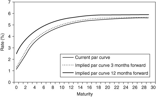
EXHIBIT 36–6
Historical Three-Month Rates and Implied Forward Rate Path Based on the Dollar Swap Curve in April 2004, June 2003, and June 2001

To add perspective, the graph also contains the historical path of the three-month rate over the past decade and the break-even path of the future three-month rates in June 2003 when monetary policy expectations were much more bullish and in June 2001 when market’s policy tightening expectations proved immature.

Forwards as Indicators of Cheap Maturity Sectors

The other ways to use forwards require less subjective judgment than the first one. As a simple example, the forward rate curve can be used to identify cheap maturity sectors visually. Abnormally high forward rates are more visible than high spot or par rates because the latter are averages of forward rates.

Exhibit 36–7 shows one real-world example from year 2000 when the par yield-curve was extremely flat (although forwards may be equally useful when the par curve is not flat). Even though the par yield-curve was almost horizontal (all par yields were within 15 basis points), the range of one-year forward rates was almost 100 basis points because the forward rate curve magnifies the cheapness/richness of different maturity sectors. High forward rates identify the 9- to 12-year sector as cheap. Forward rates are very low at the long maturities, but this characteristic probably reflects the convexity bias. Recall that forward rates are downward-biased estimates of expected returns because they ignore the convexity advantage, which is especially large at long maturities.

EXHIBIT 36–7
Par Yields and One-Year Forward Rates Based on the Dollar-Swap Curve in August 2000

Once an investor has identified a sector with abnormally high forward rates (e.g., between 9 and 12 years), she can exploit the cheapness of this sector by buying a bond that matures at the end of the period (12 years) and by selling a bond that matures at the beginning of the period (9 years). If equal market values of these bonds are bought and sold, or received and paid fixed in swaps, the position captures the cheap forward rate (in this case the 3-year rate 9 years forward). In par-curve terms, the position is exposed to a general increase in rates and a steepening yield-curve. More elaborate trades can be constructed (e.g., by selling both the 9- and 15-year bonds against the 12-year bonds with appropriate weights) to retain level and slope neutrality. To the extent that bumps and kinks in the forward curve reflect temporary local cheapness, the trade will earn capital gains when the forward curve becomes flatter and the cheap sector richens (in addition to the higher yield and rolldown the position earns).

Forwards as Relative-Value Tools for Yield-Curve Trades

Thus far in this chapter forwards are used quite loosely to identify cheap maturity sectors. A more formal way to use forwards is to construct quantitative cheapness indicators for duration-neutral flattening trades, such as barbell-bullet trades. We first introduce some concepts with an example of a market-directional trade.

When the yield-curve is upward-sloping, long-term bonds’ yield advantage over the riskless short-term bond provides a cushion against rising yields. In a sense, duration extensions are “cheap” when the yield-curve is very steep and the cushion (positive carry) is large. These trades only lose money if capital losses caused by rising rates offset the initial yield advantage. Moreover, the longer-term bonds’ rolling yield advantage¹⁷ over the short-term bond is even larger than their yield advantage. The one-year forward rate (f_{n − 1,n}) is, by construction, equal to the n-year zero’s rolling yield (see Appendix 36C). Thus it is a direct measure of the n-year zero’s rolling yield advantage. [Another forward-related measure, the change in the (n − 1)-year spot rate implied by the forwards (f_1,n − s_n−1) tells how much the yield-curve has to shift to offset this advantage and to equate the holding-period returns of the n-year zero and the one-year zero.]

Because one-period forward rates measure zeros’ near-term expected returns, they can be viewed as indicators of cheap maturity sectors. The use of such cheapness indicators does not require any subjective interest-rate view. Instead, it requires a belief, motivated by history, that an unchanged yield-curve is a good base-case scenario.¹⁸ If this is true, long-term bonds have higher (lower) near-term expected returns than short-term bonds when the forward rate curve is upward-sloping (downward-sloping). In the long run, a strategy that adjusts the portfolio duration dynamically based on the curve shape should earn higher average return than constant-duration strategies.¹⁹

Similar analysis holds for curve-flattening trades. Recall that when the yield-curve is concave as a function of duration, any duration-neutral flattening trade earns a negative carry. Higher concavity (curvature) in the yield-curve indicates less attractive terms for a flattening trade (larger negative carry) and more “implied flattening” by the forwards (that is needed to offset the negative carry). Therefore, the amount of spread change implied by the forwards is a useful cheapness indicator for yield-curve trades at different parts of the curve. If the implied change is wide historically, the trade is expensive, and vice versa.

Exhibit 36–8 shows a recent example of negative carry making curve-flattening positions expensive to hold. In October 2003, high yield-curve curvature indicated strong flattening expectations—forwards implied a 50 basis point decline in the 2- to 30-year spread over the coming six months—or high expected volatility (high value of convexity). The barbell (of the 30-year bond and six-month bill) over the duration-matched two-year bullet would become profitable only if the curve flattened even more than the forwards implied or if a sudden increase in volatility occurred. Purely on yield grounds, the two-year bullet (a steepening position) appeared cheap to the barbell. With the benefit of hindsight, we know that the carry/cheapness indicator gave a correct signal in this case. Exhibit 36–8 plots the dollar-swap curves in October 2003 and in April 2004; it is perhaps surprising that a steepening position outperformed amid curve flattening. Even though the yield-curve did flatten (the 2- to 30-year spread actually narrowed by 38 basis points by April 2004), the realized flattening did not match the forward-implied flattening. A steepener’s (bullet’s) initial carry and rolldown advantage did more than offset the capital losses owing to subsequent curve flattening.²⁰

EXHIBIT 36–8
Dollar-Swap Curves in October 2003 and in April 2004

APPENDIX 36A
Notation and Definitions

P	market price of a bond
Pn	market price of an n-year zero
C	coupon rate (in percent; other rates are expressed as a decimal)
y	annualized yield-to-maturity (YTM) of a bond
n	time-to-maturity of a bond (in years)
sn	annualized n-year spot rate; the discount rate of an n-year zero
sn−1	annualized (n − 1)-year spot rate next period; superscript * denotes next period’s (year’s) value
Δsn−1	realized change in the (n − 1)-year spot rate between today and next period()
fm,n	annualized forward rate between maturities m and n
fn−1,n	one-year forward rate between maturities (n − 1) and n; also, the n-year zero’s rolling yield
f1,n	annualized forward rate between maturities 1 and n; also called the implied (n − 1)-year spot rate one year forward
Δfn-1	implied change in the (n − 1)-year spot rate between today and next period (= f1,n − sn−1); also called the break-even yield change (over the next period) implied by the forwards
ΔfZn	implied change in the yield of an n-year zero, a specific bond, over the next period (= f1,n − Sn)
FSP	forward-spot premium (FSPn = fn−1,n − s1)
hn	realized holding-period return of an n-year zero [over one period (year)]

Rolling yield	a bond’s horizon return given a scenario of unchanged yield-curve; sum of yield and rolldown return
Bond risk premium (BRP)	expected return of a long-term bond over the next period (year) in excess of the riskless one-period bond; for the n-year zero, BRPn = E(hn − s1)
Realized BRP	realized one-year holding-period return of a long-term bond in excess of the one-year bond; also called excess bond return; realized BRPn = hn − s1
Persistence factor (PF)	slope coefficient in a regression of the annual realized BRPn on FSPn
Term spread	yield difference between a long-term bond and a short-term bond; for the n-year zero, = sn − s1
Real yield	difference between a long-term bond yield and a proxy for expected inflation; our proxy is the recently published year-on-year consumer price inflation rate
Inverse wealth	ratio of exponentially weighted past wealth to the current wealth; we proxy wealth W by the stock market level; = (Wt−1 + 0.9*Wt−2 + 0.92*Wt−3 + ⋅ ⋅ ⋅)*0.1/Wt
Duration (Dur)	measure of a bond price’s interest rate sensitivity; Dur = −(dP/dy)*(1/P)
Convexity (Cx)	measure of the nonlinearity in a bond’s P/y relation; Cx =(d2P/dy2)*(1/P)
Convexity bias (CB)	impact of convexity on the forward rate curve; CBn = −0.5*Cxn *(volatility of Δsn)2

APPENDIX 36 B
Calculating Spot and Forward Rates When Par Rates Are Known

A simple example illustrates how spot rates and forward rates are computed on a coupon date when the par curve is known (and coupon payments and compounding frequency are annual). The basis of the procedure is the fact that a bond’s price will be the same, the sum of the present values of its cash-flows, whether it is priced via yield-to-maturity—Eq. (36B.1)—or via the spot-rate curve—Eq. (36B.2).

where P is the bond price, C is the coupon rate (in percent), y is the annual yield-to-maturity (expressed as a decimal), s is the annual spot rate (expressed as a decimal), and n is the time-to-maturity (in years). We show only the computation for the first two years, which have par rates of 6% and 8%. For the first year, par, spot, and forward rates are equal (6%). Longer spot rates are solved recursively using known values of the par bond’s price and cash-flows and the previously solved spot rates. Every par bond’s price is 100 (par) by construction, so its yield (the par rate) equals its coupon rate. Because the two-year par bond’s market price (100) and cash-flows (8 and 108) are known, as is the one-year spot rate (6%), it is easy to solve for the two-year spot rate as the only unknown in the following equation:

A little manipulation shows that the solution for s₂ is 8.08%. Equation (36B.3) also can be used to compute par rates when only spot rates are known. If the spot rates are known, the coupon rate C—which equals the par rate—is the only unknown in Eq. (36B.3).

EXHIBIT 36B–1
Par, Spot, and One-Year Forward Rate Curves

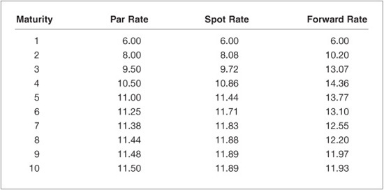
The forward rate between one and two years is computed using Eq. (36B.3) and the known one-year and two-year spot rates.

The solution for f_1,2 is 10.20%. The other spot rates and one-year forward rates (f_2,3, f_3,4, etc.) in Exhibit 36B–1 are computed in the same way. These numbers are shown graphically in Exhibit 36–1.

APPENDIX 36 C
Relations between Spot Rates, Forward Rates, Rolling Yields, and Bond Returns

Investors often want to make quick “back of the envelope” calculations with spot rates, forward rates, and bond returns. In this appendix we discuss some simple relations between these variables, beginning with a useful approximate relation between spot rates and one-year forward rates.²¹ Equation (36.2) showed exactly how the forward rate between years m and n is related to m- and n-year spot rates. Equation (36C.1) shows the same relation in an approximate but simpler form; this equation ignores nonlinear effects such as the convexity bias. The relation is exact if spot rates and forward rates are continuously compounded.

For one-year forward rates (m = n − 1), Eq. (36C.1) can be simplified to

Equation (36C.2) shows that the forward rate is equal to an n-year zero’s one-year horizon return given an unchanged yield-curve scenario: a sum of the initial yield and the rolldown return [the zero’s duration at horizon (n – 1) multiplied by the amount the zero rolls down the yield-curve as it ages]. This horizon return is often called the rolling yield. Thus the one-year forward rates proxy for near-term expected returns at different parts of the yield-curve if the yield-curve is expected to remain unchanged. We can gain intuition about the equality of the one-year forward rate and the rolling yield by examining the n-year zero’s realized holding-period return h_n over the next year, in Eq. (36C.3). The zero earns its initial yield s_n plus a capital gain/loss that is approximated by the product of the zero’s year-end duration and its realized yield change.

where is the (n – 1)-year spot rate next year. If the yield-curve follows a random walk, the best forecast for is (today’s) s_n−1. Therefore, the n-year zero’s expected holding period return is exactly the one-year forward rate in Eq. (36C.2). The key question is whether it is more reasonable to assume that the current spot rates are the optimal forecasts of future spot rates than to assume that forwards are the optimal forecasts. Empirical evidence suggests that the “random walk” forecast of an unchanged yield-curve is more accurate than the forecast implied by the forwards.

Equation (36C.2) shows that the (one-year) forward rate curve lies above the spot curve as long as the latter is upward-sloping (and the rolldown return is positive). Conversely, if the spot curve is inverted, the rolldown return is negative, and the forward rate curve lies below the spot curve. If the spot curve is first rising and then declining, the forward rate curve crosses it from above at its peak. Finally, the forward rate curve can become downward-sloping even when the spot curve is upward-sloping if the spot curve’s slope is first steep and then flattens (reducing the rolldown return). The following calculations illustrate this point and show that the approximation is good—within a few basis points from the correct values (10.20 – 13.07 – 14.36 – 13.77) in Exhibit 36B–1.

f_1,2 ≈ 8. 08+1*(8.08−6.00)=8.08+2.08=10.16;

f_2,3 ≈ 9. 72+2*(9.72−8.08)=9.72+3.28=13.00;

f_3,4 ≈ 10. 86+3*(10.86−9.72)=10.86+3.42=14.28; and

f_4,5 ≈ 11.44+4*(11.44−10.86)=11.44+2.32=13.76

KEY POINTS

• Yield-curve or the term structure of interest rates can be depicted in several interchangeable ways, including the par curve, the spot curve, and the forward rate curve.

• The main drivers of the yield-curve are the market’s rate expectations, required bond risk premiums, and convexity bias.

• A steeply upward-sloping yield-curve may reflect the market forecast of rising future short-term rates, or exceptionally high bond risk premiums, or some combination of these two. The pure expectations hypothesis assumes the first term drives yield-curve fluctuations, while empirical evidence suggests that the second term matters more. In reality, both matter.

• Forward rates can be useful tools for bond investors in break-even analysis (how much yields need to shift over a given horizon to just offset certain assets’ initial yield advantage?). and in relative value analysis (what is the expected return of a zero-coupon bond if the curve remains unchanged?).

• Treasury analysis can focus on duration extensions and yield level changes or on duration-neutral strategies and yield-curve shape changes.