CHAPTER
THIRTY-EIGHT
EMPIRICAL YIELD-CURVE DYNAMICS AND YIELD-CURVE EXPOSURE

WESLEY PHOA, PH.D.

Senior Vice President
Capital International Research, Inc.

While there are many factors that can influence the yield on a specific bond, one of the most important driving factors—especially for high-quality bonds—is the behavior of the benchmark (Treasury) yield-curve. Individual bond yields tend to move along with the yield-curve. For example, if the 10-year Treasury yield moves up or down, other bonds with maturities close to 10 years will tend to follow suit. Thus, the return on a bond portfolio is linked to movements in the Treasury yield-curve: as the yield-curve moves up and down (or tilts or changes shape in more complicated ways), the bonds in the portfolio tend to track comparable maturity Treasury yields, thus affecting the mark-to-market return of the portfolio. This sensitivity to yield-curve shifts is referred to as the yield-curve exposure or the interest rate risk of a bond or a portfolio of bonds; in order to understand and measure it, we first need to understand the ways in which the yield-curve can shift. This topic is the subject of this chapter.

FUNDAMENTAL DETERMINANTS OF YIELD-CURVE DYNAMICS

Treasury yields do not move around in a completely uncorrelated fashion. If they did, it would be impossible to analyze the interest rate risk of a bond portfolio in any meaningful way; even the notion of portfolio duration would be meaningless. Thus, in order to begin analyzing a bond portfolio, we need to make some assumption about the relationship between shifts in Treasury yields of different maturities. For example, we might try to identify the most important kinds of yield-curve shifts that can occur.

The simplest possible assumption is that all Treasury yields always move in parallel. For example, if the 30-year Treasury yield rises by 10 basis points (bp), then the 10-, five-, and two-year Treasury yields must also rise by 10 bp. Thus, all Treasury yields are perfectly correlated, and equally volatile. Under this assumption, any two Treasury bond portfolios with the same duration are equivalent. The truth is obviously more complicated than this. Bond yields need not always move in parallel, so there can be a big difference between two portfolios with the same duration. For example, if one has more of a barbell profile than the other, it will outperform if the yield-curve flattens. There is more to yield-curve risk than duration.

We need to find some way of understanding the yield-curve that recognizes that different kinds of yield-curve shifts occur, and that fits them into some systematic framework. There are at least four approaches that we could take:

1. We could make some arbitrary set of assumptions based purely on intuition; this intuition would presumably be derived from market experience.

2. We could devise a plausible mathematical model of the yield-curve and derive the possible yield-curve shifts that could occur if the model happened to conform to reality.

3. We could carry out an economic analysis of how investor expectations about economic fundamentals should drive bond yields and then identify the different kinds of shifts in the yield-curve that would result from changes in economic expectations.

4. We could look at historical shifts in Treasury bond yields and apply some statistical method to identify the different basic kinds of yield-curve shifts that have occurred in the past.

All four methods have pitfalls. Our intuitions might be wrong. There is no guarantee that a mathematical model, no matter how elegant, will be realistic. Economic arguments might be fallacious, or might overlook relevant noneconomic factors; and statistical methods often give spurious results, or even inconsistent results depending on what data is used.

In this chapter, we will adopt the following strategy. First, recognizing that investors’ economic expectations do play a large part in determining bond yields, we construct an economic argument that tells us what the yield-curve should look like and what kind of important yield-curve shifts should be possible. Next, we carry out a statistical analysis of historical Treasury bond yields, using our economic conclusions to cross-check the results and help determine which of these results are meaningful. Since we are unlikely to detect all relevant phenomena if we only use a single method of analysis, we must try to analyze the data in alternative ways.

Economic versus Noneconomic Factors in Yield-Curve Dynamics

Bond yields are determined by investor expectations. The obvious questions, then, are: What expectations are relevant? What is the precise relationship between these expectations—which are not directly observable—and observed bond yields? And finally, how does this help us understand the dynamics of the yield-curve?

It is natural to focus on economic expectations. Writing during the Depression, Keynes focused on expectations about future economic growth, demand, and output, and also about the desire for liquidity arising from uncertainty about the future—a more subtle form of expectation. Since the 1970s, it has been more fashionable to focus on expectations about future inflation, although the old Keynesian ideas have recently been revived in an attempt to understand yield-curve dynamics when the central bank is using unconventional policy tools.¹ At a minimum, both growth and inflation matter.

So we provisionally take a straightforward economic approach and simply make the assumption that forward interest rates, and thus current bond yields, are broadly determined by investors’ expectations about:

1. Real interest rates, which are determined by expected real returns on capital, and

2. Inflation, i.e., changes in the “price level”; however one wants to define that term.

Note that investors would not assume that either the real interest rate or inflation will remain constant. Both rates might be expected to rise or fall over time. However, given the lack of ability to make detailed forecasts more than one or two years forward, investors would probably assume that beyond this time horizon, both real rates and inflation tend to some long-term “equilibrium” levels when forming their expectations. The situation is pictured in Exhibit 38–1.

EXHIBIT 38–1
How economic expectations Determine expected Future Interest Rates

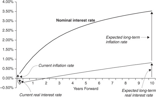
The concept of the real interest rate roughly corresponds to the real growth rate of the economy, or the real growth in output. We have not spelled out the precise relationship between expected future interest rates and current bond yields, but we assume that there is a fixed relationship between expected future interest rates and current forward rates; and of course, knowing the current forward curve is the same as knowing current bond yields. The relationship between expected future rates and forward rates actually depends on expected volatility, and the precise nature of that relationship is model-dependent. Here we simply assume that when expected future rates move, forward rates move by the same amount. This turns out to be a reasonable assumption except at extremely long forward dates.

An example may help. In our framework, the long bond yield is determined by the expected long-term real interest rate plus the expected long-term inflation rate. In the late 1980s and early 1990s, Australian long bond yields were largely driven by fluctuations in the current account deficit, which affects expectations about real interest rates. By contrast, from 1994 onward, Australian long bond yields have more often been driven by fluctuations in the Consumer Price Index (CPI), which affect investor expectations about inflation.

In the context of the U.S. bond markets, Frankel warned against focusing solely on inflationary expectations and emphasized the fact that—contrary to Fama’s assertion in 1975—real interest rates are not constant. For example, “when nominal interest rates rose sharply at the beginning of [the 1980s], it was not because expected inflation was rising. Rather contraction of monetary policy had succeeded in raising the real interest rate.”² More recently, the existence of inflation-linked Treasury securities has enabled us directly to observe fluctuations in long-term real interest rates, and these have sometimes been as volatile as long-term inflation expectations.

Note that in our framework, the slope of the yield-curve has a natural interpretation. If investors believe that real interest rates or inflation will rise from their current levels, the curve will slope upward, whereas if investors believe they will fall, it will slope downward. That is, the yield-curve has a slope because the economy is not generally believed to be in static equilibrium.

The other reason that the yield-curve might slope upward is that investors demand a risk premium for holding bonds, the so-called term premium, which rises with maturity. Empirical studies have shown that, although there does appear to be a risk premium for bonds versus Treasury bills, beyond about two years the risk premium is much less dependent on maturity (i.e., it usually has a much flatter term structure); so as a first approximation, it may be more helpful to think of the term premium as primarily consisting of a general bond market risk premium or liquidity premium versus the short term money market, rather than a duration risk premium.³

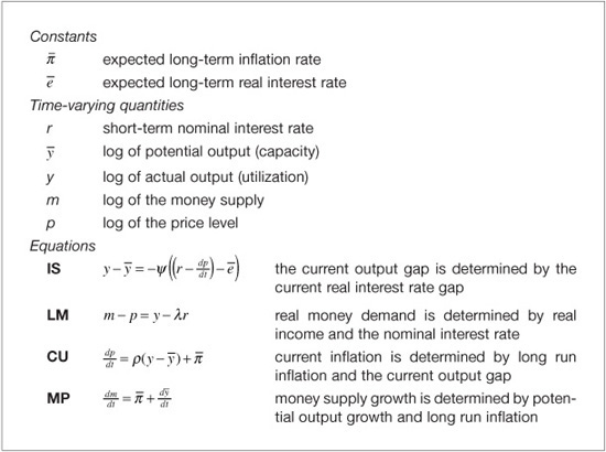
Note that the term premium is not directly observable, but must be estimated via a term structure model; and its behavior turns out to be linked to economic variables. Thus, the simple model in Exhibit 38–2 certainly does not capture all of the economic determinants of the yield-curve. But these topics are beyond the scope of this chapter.⁴

EXHIBIT 38–2
A Macro-economic Model of Adjustment in the Price Level and Interest Rates

The Shape of the Yield-Curve

Now that we have a picture of what kinds of economic expectations determine bond yields, we can go on to investigate how changes in economic expectations cause shifts in the yield-curve. It is convenient to use a simple economic model of the yield-curve originally proposed by Frankel.⁵

Let r₀ be the current short-term nominal interest rate, let be the expected long term inflation rate, and let be the expected long-term real interest rate. Then, by definition, the expected long-term nominal interest rate is + . It is usually the case that r₀ ≠ + , but it seems reasonable to assume that investors expect the future interest rate r = r_t (t > 0) to approach + as time passes. In fact, under some realistic economic assumptions, one can show that there is a constant k such that:

The macroeconomic model that Frankel used to derive this relationship is shown in Exhibit 38–2; it corresponds fairly closely with “standard undergraduate macroeconomics.” It is fairly straightforward to derive the above formula with k = ργ/(ψγ + λ;), where γ :=ψ/(1 −ψρ). However, a similar relationship appears to hold in a fairly wide variety of models of the economy, including ones that permit random shocks to the level and trend of the money supply. Thus the conclusion appears to be quite general.

The basic intuition is that interest rates take time to adjust to their expected long-term level because prices are sticky. Anyway, given r₀, the current short-term interest rate, it is easy to determine it, the expected short-term interest rate at time t:

It is convenient to write this in the form:

That is, a rational investor would expect the short-term interest rate to asymptotically approach some long-term equilibrium level + , and the expected path of future short-term rates can be described by an exponential curve. There are also other ways to arrive at this conclusion.

The economic model need not be “true” for this description of expected interest rates to hold. All we need to assume is that investors implicitly—although perhaps incorrectly—have this kind of economic model in mind when forming expectations about future interest rates. This seems to be a reasonable assumption, given the plausibility of the model and the generality of its assumptions.

The coefficients in this equation are not directly observable, but could be estimated from the current yield-curve. The term + is the expected long-term nominal interest rate in equilibrium, which will be reflected in current long bond yields, while the term ( + ) − r₀ is the spread between current nominal rates and the long-term equilibrium rate, which will be reflected in the slope of the yield-curve.

The correct interpretation of the current short term nominal interest rate r₀ is somewhat more subtle than it appears. The model describes an economy that, although not static—adjustment in interest rates takes time because prices are sticky—is moving along an equilibrium path toward a long-term steady state. This is a reasonable way to derive a medium- or long-term economic forecast, say more than two years out. In the near term, however, we know that the economy can behave in a more complex way, and we can make much more detailed forecasts about the economy that do not rely on a simple equilibrium model; the same applies to interest rates in the near term.

Thus it would be incorrect to identify r₀ with an actual current short-term interest rate, e.g., the Fed Funds rate or the three-month T-bill yield. A more appropriate interpretation, due to Richard Mason, is as follows: r₀ is “extrapolated back” from the medium- to long-term equilibrium interest rate forecasts embodied in the current yield-curve; that is, it is what the current short-term interest rate would have to be for the economy to be currently in equilibrium, i.e., to currently conform to the model. In a sense, r₀ is where the bond market thinks short-term interest rates should be, based on the economic fundamentals—and this need not coincide with their actual levels, particularly if there is disagreement between the Fed and the markets,⁶ or if the zero bound constraint is binding on short term interest rates (i.e., the optimal policy rate would otherwise be negative).

Although the interpretation seems odd at first, it is suggestive. It implies that when attempting to estimate the model, we can and should exclude money market yields from the estimation process and use only bond yields. It also tells us that any information about yield-curve shifts that the model gives us will apply to bond yields, not to money market yields.

The model predicts three kinds of observable shifts in the yield-curve:

1. Level shifts, which result from changes in the expected long-term rate + ;

2. Slope shifts, which result from changes in r₀, or rather ( + ) − r₀; and,

3. “Curvature shifts,” which result from changes in k.

In other words, level shifts arise from changes in long-term expectations; slope shifts arise from changes in expectations about monetary policy in the near term; and “curvature shifts” theoretically occur when investors believe that there has been a secular change in the economy, e.g., which makes prices inherently more sticky. The model implicitly predicts that while level shifts and slope shifts can occur all the time, “curvature shifts” should be much more rare. In fact, in the real world it is unlikely that curvature shifts occur for the economic reasons suggested by the model. Noneconomic explanations, such as supply/demand imbalances at particular points on the yield-curve, are a more plausible explanation for curvature changes. We will discuss curvature shifts further below, but for the moment we concentrate on level shifts and slope shifts.

The idea of focusing on a “long rate” and a “spread” is far from new, and all we have done here is given some theoretical justification for it. Note that so far, we have no reason to assume that level shifts and slope shifts, of the form implied by the model, should be uncorrelated. In fact, the correlation would depend on investors’ views about the nature of monetary policy. If the Fed were generally regarded as being slow to move, then a rise in long-term inflation or real rate expectations would generally be accompanied by a steepening in the yield-curve, while a fall in long bond yields would generally be accompanied by a flattening; thus the correlation would be positive.

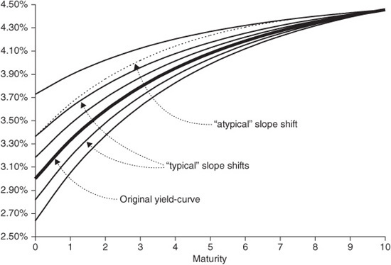
The model makes an interesting prediction about slope shifts. In periods when k is stable, all slope shifts should follow the same pattern. Slope shifts always “look the same,” except for a scaling factor. In other words, on different days one might observe slope shifts that look like any of the thin solid lines in Exhibit 38–3, but not like the thin dotted line. (The latter kind of shift is possible, but would have to be interpreted as a slope shift plus a curvature shift.) As we are about to see, this prediction is broadly consistent with the empirical data, but with some interesting qualifications.

EXHIBIT 38–3
“Typical” Yield-Curve Slope Shifts and an “Atypical” Slope Shift

EMPIRICAL ANALYSIS OF YIELD-CURVE DYNAMICS

We just used a macroeconomic model of the yield-curve to argue that shifts in bond yields should not be totally chaotic but that, since they are driven by changing economic expectations, they should be systematic and classifiable. More specifically, the most important kinds of yield-curve shifts should be level shifts and slope shifts. Can we verify this prediction by analyzing random yield-curve shifts that have occurred historically?

Using Principal Component Analysis to Identify Yield-Curve Shifts

There is a way to apply a purely statistical analysis to historical bond yields to extract “fundamental yield-curve shifts.” This was first done by Litterman and Scheinkman, using a very standard statistical method called principal component analysis.⁷ Before applying this analysis to bond yields, we briefly describe the intuition behind it by looking at a physical example taken from Jennings and McKeown.⁸ Although there are other ways to motivate principal component analysis, I think the physical analogy is an attractive one.

Consider a plank fixed to a wall. In what ways can this cantilever vibrate? It is intuitively clear that it can only vibrate at certain “natural frequencies,” or “vibration modes”; that is, any observed vibration is a combination of these vibration modes.

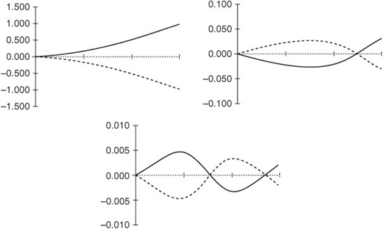
In fact, one can calculate that there are three of these modes, as shown in Exhibit 38–4. Note the scale of each of the diagrams, which indicates the relative importance of each mode: the second mode has less than a twentieth the amplitude of the first mode, and the third mode is ten times smaller again. It would probably not be visible to the naked eye.

EXHIBIT 38–4
Vibration Modes of the Cantilever

Now, suppose that we knew no physics, and wanted to work out what these vibration modes were just by observing the behavior of the plank. It is reasonable to hope that we could carry out the following procedure:

1. Attach sensors 5-, 10-, and 15-m along the plank—making the assumption that measuring the displacement of the plank at just these points gives us enough information about the whole plank.

2. Give the plank a lot of random whacks, and for each whack measure the amplitude of the observed vibration at each sensor.

3. Work out the 3 × 3 covariance matrix of these amplitudes. The diagonal will show the relative size of the displacements, whereas the other matrix elements will show whether the sensors tend to move in the same direction. In this case, all the correlations will be strongly positive, but none of them will be equal to one.

4. Extract the vibration modes by somehow “decomposing” this covariance matrix.

It turns out that if A is the covariance matrix, then the vibration modes are the eigenvectors of A, and the eigenvalues tell us how important each vibration mode is. (Recall that a vector u called an eigenvector of A, with associated eigenvalue λ, if it solves the equation Au = λu; there are standard numerical methods for finding all the eigenvectors and eigenvalues of a matrix. Also, one can prove that any two eigenvectors are orthogonal, i.e., correspond to uncorrelated modes, and in fact that the eigenvectors form an orthogonal basis.) The required “decomposition” thus amounts to finding the eigenvectors of A.

Thus, to determine the dynamics of the cantilever, it is in principle not necessary to know any physics—only matrix algebra. In practice, of course, things are unlikely to be so easy. Small measurement errors might lead to errors in the covariance matrix, and hence in the numerically computed eigenvectors and eigenvalues. The first vibration mode will be hard to miss, but the second might be difficult to detect. The third is so small, relatively speaking, that any measurement error at all will probably swamp it. Also note that since the eigenvectors are orthogonal by construction, they correspond to uncorrelated or independent vibration modes.

We can apply exactly the same method to analyzing the dynamics of the yield-curve: identify some “key points” (standard bond maturities that represent key liquidity points); look at historical yield shifts at each of these points; compute the covariance matrix of yield shifts; and compute its eigenvectors and eigenvalues. Each eigenvector should correspond to a fundamental yield-curve shift, and by definition these fundamental shifts are uncorrelated. The eigenvalues are weights, which tell us the relative importance of each of these shifts; and the actual yield-curve shift on any specific day is a linear combination of fundamental shifts.

Our economic analysis might lead us to expect that the most important fundamental shift will turn out to be a parallel shift, whereas the second most important will turn out to be a slope shift. But we are not certain that this will be the case; for example, since the parallel and slope shifts predicted by the model are not necessarily uncorrelated, they will both turn out to be linear combinations of the fundamental shifts identified by the statistical analysis, which are by definition uncorrelated. However, since the correlation is low, we might hope that the two most important fundamental shifts would closely resemble a parallel shift and a slope shift.

Note that on its own the economic analysis tells us nothing about the relative importance of these two different kinds of yield-curve shift; and we do not know what other kinds of shifts there might be. Here the statistical analysis should yield some valuable insights. However, since the results of this empirical analysis might depend on the dataset used, it is important to test their robustness by running the analysis on a variety of datasets.

The results of a principal component analysis may depend on which bond yields we feed into the analysis. For example, if we include a large number of money market yields, we are more likely to pick up yield-curve shifts specifically affecting the money market curve, and we will give a lower weighting to yield-curve shifts affecting midrange bonds, or perhaps fail to detect such shifts at all. Thus, as with any statistical analysis, we must be careful to select the most “relevant” observables. For most bond investors, this means using bond yields in preference to money market yields.

Finally, a technical point: We use the correlation matrix rather than the covariance matrix in our analysis. This corresponds to scaling away differences in yield volatility at different points in the yield-curve.⁹ The fundamental yield shifts identified by a principal component analysis of U.S. Treasury yields are shown in Exhibit 38–5. Only the first four eigenvectors are shown; the others have negligibly small weights. One can make the following remarks about these empirically observed fundamental yield-curve shifts:

EXHIBIT 38–5
Principal Component Analysis of U.S. Treasury Yields, 1993–2011

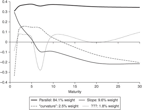
1. The dominant fundamental shift is an empirical level shift (thick solid line), a nearly parallel shift in yields across the whole curve. This explains around 85% of observed variation in yields.

2. The next most important fundamental shift is an empirical slope shift [thin solid line], in which the yield-curve pivots around the five-year point. This explains around 10% of observed variation in yields, and seems to have become slightly more important in recent years.

3. The third most important fundamental shift is an empirical curvature shift (dashed line), sometimes called a “butterfly shift,” in which three-to six-year bond yields move relative to shorter and longer bonds. The precise nature and importance of a curvature shift seems to vary from period to period, and curvature shifts explain less than 3% of observed yield shifts.

4. The remaining shifts identified by the principal component analysis—such as the fourth eigenvector, the only remaining one that is shown in the exhibit (as a dotted line)—seem to have no meaningful interpretation, and are probably due to statistical noise. They vary depending on the dataset.

How robust are these findings? One important check is to determine whether the observed dynamics have varied over time. We can do this by carrying out the same analysis using different time periods; this is done in the three panels of Exhibit 38–6, which compare the first, second, and third eigenvalues (i.e., level, slope, and curvature shifts) observed in five different time periods, corresponding to different monetary policy regimes in the United States:

EXHIBIT 38–6A
Parallel Shifts in U.S. Treasury Curves, Different Time Periods

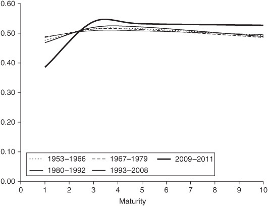
EXHIBIT 38–6B
Slope Shifts in U.S. Treasury Curves, Different Time Periods

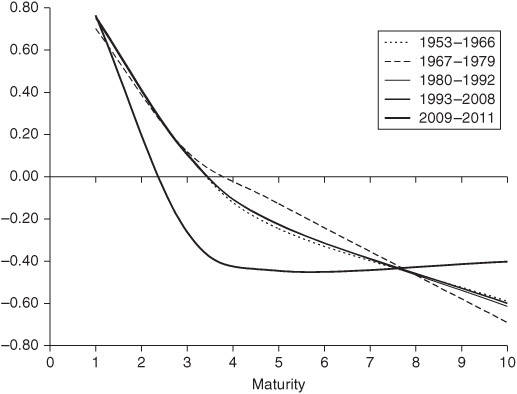
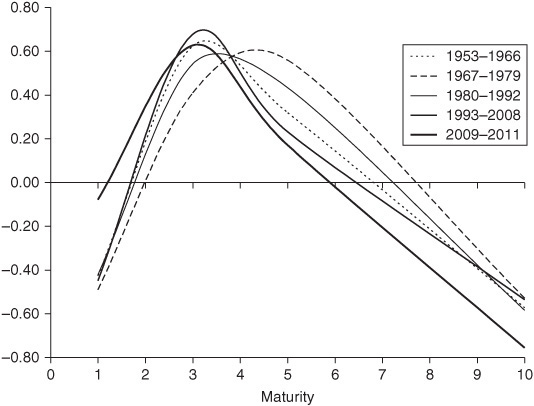
EXHIBIT 38–6C
“Curvature Shifts” in U.S. Treasury Curves, Different Time Periods

• 1953–1966: A period of low inflation and conservative Fed policy, largely under Chairman Martin

• 1967–1979: A period of loose monetary policy and accelerating inflation, under Burns and Miller

• 1980–1992: A period of tight monetary policy and disinflation, under Volcker (including an initial period in which monetary aggregates were being targeted aggressively)

• 1993–2008: A period of moderate inflation and conventional Fed policy, under Greenspan and Bernanke (involving fed funds targeting broadly consistent with the Taylor rule, and with increasing transparency over time)

• 2009–2011: A period of near-zero short-term interest rates with a binding zero bound, and unconventional Fed policy under Bernanke (involving a large expansion of the Fed’s balance sheet), following the global financial crisis

The results can be broadly summarized as follows:

• In all periods, the three most important eigenvectors seem to correspond to level, slope, and curvature shifts.

• The importance of the level shift is fairly constant over time, with a weight over 90% in all periods except the last, in which the weight is around 82%. The shape of the level shift is also fairly constant over time, being nearly parallel in every period except the last, in which it involves a smaller shift at the short end of the curve. This presumably reflects the fact that the short end of the curve was pinned by the zero interest rate target.

• The importance of the slope shift is fairly constant over time, with a weight between 5% and 10% in all periods except the last, in which the weight is around 15%. The shape of the slope shift is remarkably constant over time, except in the last period.

• The weight of the “curvature” shift is less than 4% in all periods, and the peak of the hump varies in different periods, moving between the three- and five-year part of the curve.

It is tempting to conclude that because parallel shifts account for such a large proportion of variance in Treasury yields, slope shifts and other kinds of shifts are not important. This is incorrect. The reason is that most bond investors are evaluated against a benchmark rather than on the basis of total return. An investor who is tracking benchmark duration closely has, by definition, nearly the same exposure to parallel shifts as the benchmark; but exposure to yield-curve slope may be quite different; for example, if the portfolio has a barbell profile. In this case yield-curve slope shifts would play a major role, sometimes the primary role, in determining relative performance.

Incidentally, the appearance of level, slope, and curvature shifts in the analysis are not empirical accidents. Lord and Pelsser show that they follow from mathematical properties of the correlation matrix.¹⁰ For example, if all the correlations are positive then the most important eigenvalue will always be a level shift, in the sense that yields at all maturities move in the same direction; and if the correlation curves become flatter for longer maturities (Exhibit 38–9), then the second most important eigenvalue will be a slope shift. However, this says nothing about the shape of these shifts; for example, it does not tell us that the level shift must be parallel rather than having a more complex shape as it did in the case of the U.S. Treasury curve in the 2009–2011 period. So the mathematics does not obviate the need to carry out the principal components analysis.

Our analysis so far has focused on the U.S. Treasury market. It is logical to ask whether similar results hold for other bond markets—and also whether the apparent change in behavior in the most recent period has any analog in different markets. Since the earlier arguments about how interest rate expectations determine the shape of the yield-curve should apply equally to most market economies, one would expect the term structure dynamics in different developed countries to be broadly similar. This turns out to be the case, although there are minor differences that have an interesting interpretation.

Exhibit 38–7a shows the results of a principal components analysis carried out on Euro Area Government bond yields (specifically, the German bund curve). The results are quite similar to the full period U.S. Treasury analysis, although the hump of the “curvature” shift seems to occur at a longer maturity point. Note that the level shift is nearly parallel in nature.

EXHIBIT 38–7A
Principal Component Analysis of Euro Area Government Bond Yields, 2000–2011

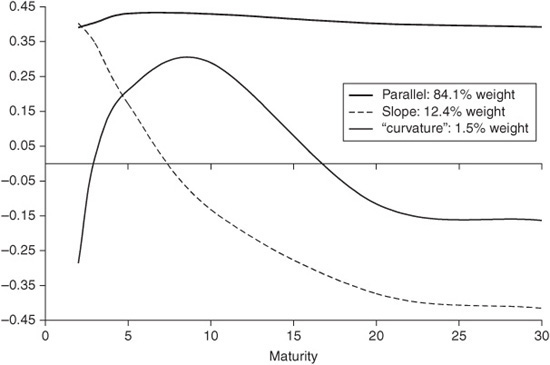
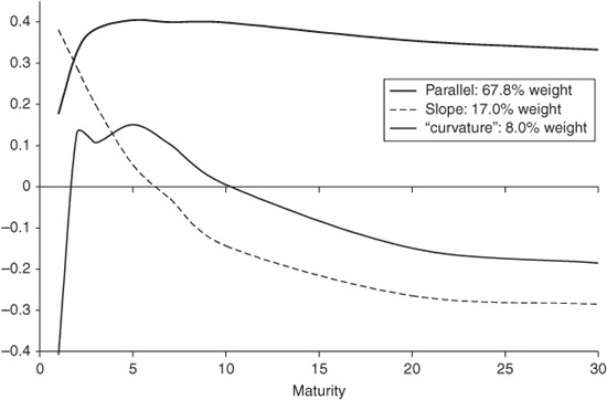
Exhibit 38–7b shows the results of a principal components analysis carried out on Japanese Government bond yields. The results are quite similar to the U.S. Treasury analysis during the period 2009–2011, with a comparable downward bend at the short end of the level shift. This is unsurprising, since during the period analyzed, the zero bound was also binding on the Bank of Japan’s short-term interest rate target, and it was engaged in unconventional monetary policy (quantitative easing) during much of this period.¹¹

EXHIBIT 38–7B
Principal Component Analysis of Japanese Government Bond Yields, 2000–2011

Overall, we can conclude that:

1. Level and slope shifts, taken together, do a good job at describing the bulk of yield-curve risk.

2. “Curvature” shifts explain much of the rest, but the nature of a curvature shift is more elusive.

3. Yield-curve dynamics may be a little different during periods of unconventional monetary policy, or when the zero bound is binding.

Implications for Portfolio Risk Management

It has been argued that if level shifts are not parallel, then duration is an inappropriate portfolio risk measure. The effective duration of a portfolio measures its sensitivity to a parallel shift in the yield-curve; arguably, it should be replaced with a “level duration” that measures its sensitivity to the empirical level shift, which is not perfectly parallel. The natural counterargument is that duration is more widely understood and easier to calculate. Moreover, since a U.S. level shift is approximately parallel, one would get a similar answer anyway. Note that for maturities of three years and greater, even level shifts in periods of unconventional monetary policy look roughly parallel. It is only shorter maturities that don’t move in parallel. Thus, even under these conditions, a parallel shift is a reasonable proxy for a level shift when one is analyzing portfolios which do not contain many short maturity bonds.

On a more fundamental level, we argued earlier in this chapter that if we interpret yield-curve shifts as arising mostly from changes in economic expectations, it is natural to focus on parallel shifts and slope shifts—in which “slope” refers to the spread between the short rate and the long bond yield. We also observed that there was no reason to expect these parallel shifts and slope shifts to be uncorrelated. Now the factors identified by a principal component analysis must, by definition, be uncorrelated. This means that the first two principal components—the empirical level and slope shifts—should be interpreted as certain linear combinations of the economically meaningful parallel and slope shifts. That is, the fact that the empirical factors are forced to be uncorrelated means that they may not be intrinsically meaningful.

For example, if inflation is unusually volatile and there is a high correlation between rises in inflationary expectations and monetary tightenings—that is, if tightenings tend to occur in response to market perceptions of inflationary pressures, and to overshoot them—the empirical level shift would not look parallel. Thus the nature of the empirical level shift—unlike the economically meaningful parallel and slope shifts—depends on whether unusual economic circumstances may have influenced monetary policy during the period being studied.

When monitoring interest rate risk, it is preferable to focus on economically meaningful parallel shifts and slope shifts, which may have non-zero correlation, rather than the empirical level shifts and slope shifts identified by principal component analysis. That is, rather than constructing new risk measures from the principal components, one should continue to use duration, and supplement it with a “slope duration” derived from the economic analysis.

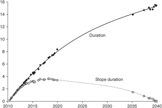
Note that unlike parallel duration, there is no “standard” definition of slope duration. A convenient definition of “slope duration” might be calculated as follows: Let a “slope shift” correspond to a shift with the same shape as the second principal component in Exhibit 38–5, but translated and scaled so that the two-year point shifts by 100 bp and the 30-year point remains unchanged. (It should also be smoothed somewhat.) Given a bond, compute its value after this slope shift has been applied to the current yield-curve. The percentage change from the original price is the slope duration of the bond.

Other definitions are possible. For example, one could alternatively let a “slope shift” be any of the empirical slope shifts shown in Exhibit 38–6b, and the chosen shift could be translated and scaled so that the six-month yield moves by 100 bps and the 10-year yield remains unchanged. The precise choice doesn’t matter as long as it’s applied consistently. The important thing is to apply a consistent definition of slope shift to different bonds, and at different times.

Exhibit 38–8 shows ordinary durations and slope durations for outstanding noncallable Treasury bonds, using our suggested definition of slope duration. (The graphs are not perfectly smooth curves because of the differing bond coupon rates.) Note that while parallel duration rises with maturity, slope duration is highest for bonds with a maturity of around seven years. The reason is that the yields of longer bonds are not greatly affected by a yield-curve slope shift.

EXHIBIT 38–8
Ordinary (Parallel) Durations and Slope Durations of Selected Noncallable Treasuries

A word on curvature shifts and other less significant yield-curve shifts (such as “hump shifts,” curvature shifts affecting very short maturities when these are included in the data set). These crop up persistently in principal component analyses, and thus it is tempting to regard them as “fundamental” factors on a par with level and slope shifts—but that happen to be much less important. This is not quite the case. As we saw earlier in this chapter, level and slope shifts have a natural economic meaning, and the form of a level shift or a slope shift tends to be quite stable over time.

By contrast, a curvature shift or a hump shift generally has no economic interpretation, and the region of the yield-curve most affected by such a shift can vary widely. For example, a hump in the money market curve is usually the result of a sophisticated market prediction about future monetary policy, and might center on around (say) the 9-, 12-, or 18-month part of the yield-curve, depending on circumstances Similarly, curvature shifts generally arise because of supply/demand imbalances that affect very particular parts of the yield-curve. For example, in late 1995, three-year Australian Government bond yields were driven down by swap market activity arising from Australian issuance in the Japanese market and from specific deals related to the privatization of the Victorian power industry; three-year yields were specifically affected because of Japanese retail demand for three-year investments and because of the nature of the privatization deals being arranged. In different circumstances it might have been the two-, or five-year, part of the curve that was most affected. It was not useful to regard this phenomenon as a “curvature shift” in some generic sense.

The practical conclusion for portfolio risk management is as follows. It makes sense to measure portfolio “level risk” and “slope risk” in a consistent way, as these correspond to fundamental interest rate risk factors. The meaning of a level shift or a slope shift does not change over time. However, it is not advisable to take an equally rigid approach to measuring “curvature risk” or “hump risk,” since curvature or hump shifts do not have any fundamental significance, but occur for more specific reasons, and take different forms at different times. Thus, one must adopt a more flexible approach to monitoring this kind of yield-curve reshaping risk. We will explore this further later in the chapter.

BEYOND LEVEL AND SLOPE RISK

It was just suggested that, when monitoring overall portfolio interest rate risk, it is most important to focus on parallel duration and slope duration. For example, these two risk measures capture the effects of long/short duration bets, and of steepening/flattening trades. Since the other principal components have such a low weight, and we argued that measuring curvature risk and hump risk was problematic, one might think that only parallel and slope risk matter. Unfortunately, this is not quite the case. In practice, these two risk factors are not comprehensive.

Empirical Correlations versus Theoretical Correlations

There is a certain kind of risk that is obscured by principal component analysis: the risk that, perhaps for an event-specific reason, a specific part of the yield-curve will shift. The behavior of the three-year part of the Australian yield-curve in late 1995, discussed above, is an example. This had a significant impact on bond returns during that period. But if this precise yield-curve shift did not happen repeatedly, it would not appear statistically significant when carrying out a principal component analysis using five or ten years of data. A more recent example would be the behavior of the five-year U.S. Treasury note during 2010, as it richened dramatically relative to other maturities, then cheapened even more rapidly.

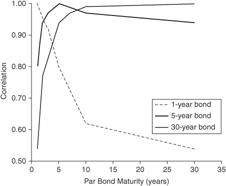
How can we determine what is lost when we focus only on parallel duration and slope duration? To answer this question, Rebonato and Cooper compared (a) the empirical correlations of changes in different bond yields, with (b) the correlations predicted if only parallel shifts and slope shifts had occurred.¹²

Exhibit 38–9 shows empirical correlations for one-, five-, or 30-year Treasury yield as a function of the yield to which this is being compared. For example, the five-year yield has a correlation of around 0.95 with both the three-and seven-year yield, but only 0.90 with the 30-year yield and only 0.85 with the one-year yield. Note that the correlations fall away sharply as we move away from the specified bond.

EXHIBIT 38–9
empirical Correlations of Different Treasury Yields

Exhibit 38–10 shows what these correlations would have been if only parallel shifts and slope shifts had occurred. Note that they fall away much more gradually as we move away from the specified bond. That is, the theoretical correlation between nearby bonds is much higher than the empirical correlation. This shows that focusing only on parallel risk and slope risk understates the basis risk between two nearby bonds; it suggests that (say) the five-year bond and the seven-year bond should be much closer substitutes than they actually are.

EXHIBIT 38–10
Theoretical Correlations of Different Treasury Yields, Two Factor Model

The pattern of gradually declining correlations observed in Exhibit 38–10 is not an accident. Rebonato and Cooper proved mathematically that if you assume only two kinds of yield-curve shift, the correlation functions must behave like this. This may be viewed as a kind of converse to the results of Lord and Pelsser mentioned earlier.

What is the appropriate way to monitor maturity-specific risks that do not correspond to fundamental yield-curve shifts that occur repeatedly? At the moment, the most useful tool seems to be the concept of partial duration, which measures exposure to a yield change at a single point on the yield-curve. We briefly review this concept. To compute, for example, a five-year partial duration, shift the five-year point of the yield-curve by 100 bps, and recompute the value of the bond. The percentage change from the original price is the partial duration.¹³ (There are other possible definitions. For example, it is also common to apply a shift to the zero coupon yield-curve rather than the benchmark or par yield-curve. There is also no standard set of maturity points used to calculate partial durations.)

There are a number of important observations to make about the concept of partial duration:

• The yield-curve shifts used in the definition of partial duration are not economically meaningful; in fact, they are highly unrealistic. Therefore, single partial durations do not have any economic interpretation, and are purely tools, “building blocks” of yield-curve risk.

• The definition of a specific partial duration may depend on the set of yield-curve maturity points chosen. For example, the value and meaning of the 10-year partial duration will differ depending on whether the adjacent grid points are at 5 and 30 years, or at 7 and 20 years.

• The definition of a specific partial duration also depends on how yields are interpolated between maturity points. The above examples assume linear interpolation, but different methods could be used.

• Care must be taken when computing partial durations for securities with interest-rate sensitive cash flows, particularly adjustable-rate mortgages (ARMs) with reset caps or floors. This is because shifting a single maturity point of the observed yield-curve corresponds to a much more complex and extreme displacement in the forward curve, and since cap and floor valuation is highly sensitive to the forward curve, the results can be numerically unstable.

These observations partly explain why partial durations can often look somewhat unintuitive. Parallel and slope durations are easy to interpret, whereas interpreting partial durations takes some experience. Exhibit 38–11 shows examples of partial durations for some different kinds of securities. Ordinary (parallel) durations and slope durations are also shown, and securities with similar durations are grouped together. Here are some observations about these numbers:

EXHIBIT 38–11
Comparison of Yield-Curve Risk Measures for Different Security Types

• Compared with bonds with more concentrated cash flows, bonds with spread-out cash flows have lower slope duration and have partial durations that are more spread out over the maturity points used. “Bonds with more spread-out cash flows” include bonds with higher coupons and amortizing bonds.

• The same applies to callable bonds, whose cash flows are “spread out” in the sense that they vary in different interest rate environments. Thus, the callable municipal bond with a 30-year maturity and a 10-year call date has partial durations at both of those maturity points, and lower slope duration than the comparable duration serial.

• A fortiori, the same also applies to mortgage pools, which are both amortizing and have option-like cash flows, varying under different interest rate environments due to different prepayment speeds.

Partial durations permit investors to match yield-curve exposures very precisely, and are particularly useful in asset/liability management. However, the precise way in which partial durations are used vary from investor to investor. In fact, a useful application of partial durations is to compute approximate sensitivities to arbitrary yield-curve shifts, such as those identified by a principal component analysis.

Various methods have been proposed for computing “yield-curve reshaping durations” in specific cases; for example, the approach of Willner¹⁴ represents yield-curve displacements using an explicit functional form, following Nelson and Siegel.¹⁵ Implementing this approach on a portfolio level involves considerable additions and modifications to one’s existing portfolio analytical system. Also, it is not obvious how to measure exposure to an arbitrary reshaping; for example, different kinds of curvature shift, or the nonparallel level shifts observed in periods of unconventional monetary policy.

There is a more straightforward method for computing the sensitivity of a bond or bond portfolio to an arbitrary yield-curve reshaping. For any given reshaping, this exposure is approximately equal to a fixed linear combination of the bond’s partial durations. This suggests that it may be better to regard partial durations as providing a general tool for decomposing arbitrary “relevant” or “meaningful” yield-curve reshapings.

Idiosyncratic Behavior at the Short End of the Curve

The analysis of correlations showed that there are maturity-specific risks not captured by parallel risk and slope risk. There are two other sources of additional risk: “money market risk” and “long end risk.” These arise because both the short and long ends of the curve can move independently of the 2- to 10-year section of the yield-curve. Note that idiosyncratic shifts in the short or long end of the curve may not be detected by the principal component analysis unless several observations from the short or long end of the curve are included. For example, if the dataset for a principal components analysis only includes a single long bond yield observation, a statistically significant “long end” factor is unlikely to be detected. Similarly, the dynamics of the very short end of the yield-curve is not likely to be well described by an analysis that uses very few maturity points in that region of the curve. (Recall also that the theoretical analysis of yield-curve dynamics at the beginning of this chapter should not be expected to tell us much about dynamics at the very short end of the curve.)

Note that the precise behavior of money market yields may vary widely from country to country, depending on central bank operating procedures and other idiosyncratic factors. For example, the monetary authorities in the United States and Australia attempt to make relatively smooth adjustments in monetary policy, thus the very short end of the curve (0–three months) is often less volatile than longer money market yields (say, 6–18 months). On the other hand, the Reserve Bank of New Zealand had at times often permitted much more volatility in overnight to three-month yields. The point is that, while the economic factors driving bond yields are generally the same in different countries, the factors driving money market yields are not. They depend on the character of monetary policy in each country.

When attempting to analyze the behavior of money market yields, it is important to take two precautions. First, because rates corresponding to maturities of less than one month have extremely volatile yields, these should usually be excluded from any statistical analysis. Second, because the behavior of the short end of the curve depends on the current character of monetary policy, it does not make sense to use datasets spanning several monetary regimes.

Bearing this in mind, Exhibit 38–12 focuses purely on the short end. It shows the results of a principal components analysis carried out on LIBOR rates with maturities from one to 12 months. Note that:

EXHIBIT 38–12
Principal Component Analysis of USD LIBOR Rates, 1991–2011

• The analysis identifies level, slope and curvature shifts as before.¹⁶ However, the level shift is not perfectly parallel. This is observed using a 20-year analysis period, so it is not due to the fact that Fed policy was unconventional. Rather, it is probably due to inertia in very short-term interest rates. The Fed tends to make only gradual changes to overnight rates.

• And, the “curvature shift” peaks at the three-month maturity point, so it is obviously unrelated to the “curvature shift” observed in the analysis of U.S. Treasury curve dynamics.

It is hard to draw any definitive conclusions about the dynamics of short maturity yields, particularly since a shift in the nature of monetary policy may make any previous conclusions invalid. Probably the best one can do is to monitor carefully chosen partial durations. In any case, the dollar risk is much lower than for bonds, and investors often have much less flexibility in their money market holdings than in their bond holdings; so in practice there is perhaps more tolerance for error.

As an aside, note that many empirical studies of interest rate dynamics have focused solely on T-bill yields. The above analysis shows that the relevance of such studies to understanding bond yields is dubious. The bond curve must be analyzed separately from the money market curve.

KEY POINTS

• Yield-curve shifts are not always parallel. It is thus inadvisable to use the conventional notion of duration as the only measure of interest rate risk.

• Both theoretical and empirical analyses suggest that the two most important kinds of yield-curve shift are parallel shifts and slope shifts.

• The forms of these shifts can be identified empirically using principal components analysis. They are more or less uniform over time, except during periods when short-term interest rates are at the zero bound.

• The risk measures corresponding to these two kinds of yield-curve shift are conventional (parallel) duration and slope duration. Taken together, these capture most but not all of a portfolio’s yield-curve risk exposure.

• “Curvature shifts” appear to be important, but do not have a clear economic interpretation and are less uniform over time; a better way to monitor exposure to more complex yield-curve shifts is via partial durations.