
CHAPTER
FORTY
VALUATION OF BONDS WITH EMBEDDED OPTIONS
FRANK J. FABOZZI, PH.D., CFA, CPA
Professor of Finance
EDHEC Business School
ANDREW KALOTAY, PH.D.
President
Andrew Kalotay Associates
MICHAEL DORIGAN, PH.D.
Director & Senior Quantitative Analyst
PNC Capital Advisors LLC
The complication in building a model to value bonds with embedded options and option-type derivatives is that cash flows will depend on interest rates in the future. Academicians and practitioners have attempted to capture this interest rate uncertainty through various models, often designed as single or multi-factor models. These models attempt to capture the stochastic behavior of rates.
In practice, these elegant mathematical models must be converted to numeric applications. Here we focus on one such model—a single-factor model that assumes a stationary variance or, as it is more often called, volatility. We demonstrate how to move from the yield curve to a valuation lattice. Effectively, the lattice is a representation of the model, capturing the distribution of rates over time. In our illustration we will present the lattice as a binomial tree, the most simple lattice form.
The lattice holds all the information required to perform the valuation of certain option-like interest rate products. First, the lattice is used to generate cash flows over the life of the security. Next, the interest rates on the lattice are used to compute the present value of those cash flows.
There are several interest rate models that have been used in practice to construct an interest rate lattice. These are described in other chapters. In each case, interest rates can realize one of several possible rates when we move from one period to the next. A lattice model where it is assumed that only two rates are possible in the next period given the current rate is called a binomial model. A lattice model where it is assumed that interest rates can take on three possible rates in the next period is called a trinomial model. There are even more complex models that assume more than three possible rates in the next period can be realized.
Regardless of the underlying assumptions, each model shares a common restriction. The interest rate tree generated must produce a value for an on-the-run optionless issue that is consistent with the current par yield curve. In effect, the value estimated by the model must be equal to the observed market price for the optionless instrument. Under these conditions, the model is said to be “arbitrage free.” A lattice that produces an arbitrage-free valuation is said to be “fair.” The lattice is used for valuation only when it has been calibrated to be fair. More on calibration below.
In this chapter we show how to value bonds with embedded options using the lattice methodology. We begin by demonstrating how an interest rate lattice is constructed. Then we use the model to value bonds with an embedded option. The lattice methodology also can be used to value floating-rate securities with option-type derivatives, options on bonds, caps, floors, swaptions, and forward-start swaps.1
THE INTEREST RATE LATTICE
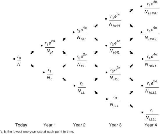
Exhibit 40–1 provides an example of a binomial interest rate tree, which consists of a number of “nodes” and “legs.” Each leg represents a one-year interval over time. A simplifying assumption of one-year intervals is made to illustrate the key principles. The methodology is the same for smaller time periods. In fact, in practice, the selection of the length of the time period is critical, but we need not be concerned with this nuance here.
EXHIBIT 40–1
Four-Year Binomial Interest Rate Tree

The distribution of future interest rates is represented on the tree by the nodes at each point in time. Each node is labeled as N and has a subscript, a combination of L’s and H’s. The subscripts indicate whether the node is lower or higher on the tree, respectively, relative to the other nodes. Thus node NHH is reached when the one-year rate realized in the first year is the higher of the two rates for that period, then the highest of the rates in the second year.
The root of the tree is N, the only point in time at which we know the interest rate with certainty. The one-year rate today (i.e., at N) is the current one-year spot rate, which we denote by r0.
We must make an assumption concerning the probability of reaching one rate at a point in time. For ease of illustration, we have assumed that rates at any point in time have the same probability of occurring; in other words, the probability is 50% on each leg.
The interest rate model we will use to construct the binomial tree assumes that the one-year rate evolves over time based on a log-normal random walk with a known (stationary) volatility. Technically, the tree represents a one-factor model. Under the distributional assumption, the relationship between any two adjacent rates at a point in time is calculated via the following equation:
![]()
where σ is the assumed volatility of the one-year rate, t is time in years, and e is the base of the natural logarithm. Since we assume a one-year interval, that is, t = 1, we can disregard the calculation of the square root of t in the exponent.
For example, suppose that r1,L is 4.4448% and σ is 10% per year, then
![]()
In the second year, there are three possible values for the one-year rate. The relationship between r2,LL and the other two one-year rates is as follows:
![]()
Thus, for example, if r2,LL is 4.6958%, and assuming once again that σ is 10%, then
r2,HH = 4.6958%(e4×0.10) = 0 7.0053%
and
r2,HL = 4.6958%(e2×0.10) = 5.7354%
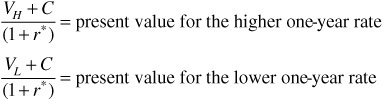
This relationship between rates holds for each point in time. Exhibit 40–2 shows the interest rate tree using this new notation.
EXHIBIT 40–2
Four-Year Binomial Interest Rate Tree with One-Year Rates*
Determining the Value at a Node
In general, to get a security’s value at a node, we follow the fundamental rule for valuation: The value is the present value of the expected cash flows. The appropriate discount rate to use for cash flows one year forward is the one-year rate at the node where we are computing the value. Now there are two present values in this case: the present value of the cash flows in the state where the one-year rate is the higher rate and one where it is the lower-rate state. We have assumed that the probability of both outcomes is equal. Exhibit 40–3 provides an illustration for a node assuming that the one-year rate is r* at the node where the valuation is sought and letting
EXHIBIT 40–3
Calculating a Value at a Node
VH = the bond’s value for the higher one-year rate state
VL = the bond’s value for the lower one-year rate state
C = coupon payment
From where do the future values come? Effectively, the value at any node depends on the future cash flows. The future cash flows include (1) the coupon payment one year from now and (2) the bond’s value one year from now, both of which may be uncertain. Starting the process from the last year in the tree and working backwards to get the final valuation resolves the uncertainty. At maturity, the instrument’s value is known with certainty—par. The final coupon payment can be determined from the coupon rate or from prevailing rates to which it is indexed. Working back through the tree, we realize that the value at each node is calculated quickly. This process of working backward is often referred to as recursive valuation.
Using our notation, the cash flow at a node is either
VH + C for the higher one-year rate
VL + C for the lower one-year rate
The present value of these two cash flows using the one-year rate at the node, r*, is
Then the value of the bond at the node is found as follows:
![]()
CALIBRATING THE LATTICE
We noted earlier the importance of the no-arbitrage condition that governs the construction of the lattice. To ensure that this condition holds, the lattice must be calibrated to the current par yield curve, a process we demonstrate here. Ultimately, the lattice must price optionless par bonds at par.
Assume the on-the-run par yield curve for a hypothetical issuer as it appears in Exhibit 40–4. The current one-year rate is known, 3.50%. Hence the next step is to find the appropriate one-year rates one year forward. As before, we assume that volatility σ is 10% and construct a two-year tree using the two-year bond with a coupon rate of 4.2%, the par rate for a two-year security.
EXHIBIT 40–4
Issuer Par Yield Curve

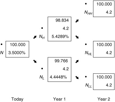
Exhibit 40–5 shows a more detailed binomial tree with the cash flow shown at each node. The root rate for the tree r0 is simply the current one-year rate, 3.5%. At the beginning of year 2, there are two possible one-year rates, the higher rate and the lower rate. We already know the relationship between the two. A rate of 4.75% at NLh has been chosen arbitrarily as a starting point. An iterative process determines the proper rate (i.e., trial-and-error). The steps are described and illustrated below. Again, the goal is a rate that, when applied in the tree, provides a value of par for the two-year 4.2% bond.
Step 1. Select a value for r1. Recall that r 1 is the lower one-year rate. In this first trial, we arbitrarily selected a value of 4.75%.
Step 2. Determine the corresponding value for the higher one-year rate. As explained earlier, this rate is related to the lower one-year rate as follows: rle2σ. Since r1 is 4.75%, the higher one-year rate is 5.8017% (= 4.75% e2×0.10). This value is reported in Exhibit 40–5 at node NH.
EXHIBIT 40–5
The One-Year Rates for Year 1 Using the Two-Year 4.2% On-the-Run Issue: First Trial
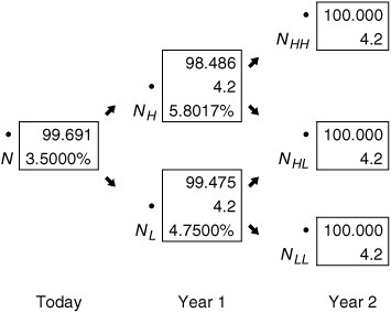
Step 3. Compute the bond value’s one year from now. This value is determined as follows:
a. Determine the bond’s value two years from now. In our example, this is simple. Since we are using a two-year bond, the bond’s value is its maturity value ($100) plus its final coupon payment ($4.2). Thus it is $104.2.
b. Calculate VH. Cash flows are known. The appropriate discount rate is the higher one-year rate, 5.8017% in our example. The present value is $98.486 (= $104.2/1.058017).
c. Calculate VL. Again, cash flows are known—the same as those in step 3b. The discount rate assumed for the lower one-year rate is 4.75%. The present value is $99.475 (= $104.2/1.0475).
Step 4. Calculate V.
a. Add the coupon to both VH = and VL to get the cash flow at NH and NL, respectively. In our example we have $102.686 for the higher rate and $103.675 for the lower rate.
b. Calculate V. The one-year rate is 3.50%. (Note: At this point in the valuation, r* is the root rate, 3.50%). Therefore, $99.691 = 1/2($99.214 + $100.169)
Step 5. Compare the value in step 4 to the bond’s market value. If the two values are the same, then the rl used in this trial is the one we seek. If, instead, the value found in step 4 is not equal to the market value of the bond, this means that the value rl in this trial is not the one-year rate that is consistent with the current yield curve. In this case, the five steps are repeated with a different value for rl.
When rl is 4.75%, a value of $99.691 results in step 4, which is less than the observed market price of $100. Therefore, 4.75% is too large, and the five steps must be repeated trying a lower rate for rl.
Let’s jump right to the correct rate for rl in this example and rework steps 1 through 5. This occurs when rl is 4.4448%. The corresponding binomial tree is shown in Exhibit 40–6. The value at the root is equal to the market value of the two-year issue (par).
EXHIBIT 40–6
The One-Year Rates for Year 1 Using the Two-Year 4.2% On-the-Run Issue
We can “grow” this tree for one more year by determining r2. Now we will use the three-year on-the-run issue, the 4.7% coupon bond, to get r2 . The same five steps are used in an iterative process to find the one-year rates in the tree two years from now. Our objective is now to find the value of r 2 that will produce a bond value of $100. Note that the two rates one year from now of 4.4448% (the lower rate) and 5.4289% (the higher rate) do not change. These are the fair rates for the tree one-year forward.
The problem is illustrated in Exhibit 40–7. The cash flows from the three-year 4.7% bond are in place. All we need to perform a valuation are the rates at the start of year 3. In effect, we need to find r2 such that the bond prices at par. Again, an arbitrary starting point is selected, and an iterative process produces the correct rate.
The completed version of Exhibit 40–7 is found in Exhibit 40–8. The value of r2 , or equivalently r2,LL, that will produce the desired result is 4.6958%. The corresponding rates r 2,HL and r2,HH would be 5.7354% and 7.0053%, respectively.
EXHIBIT 40–7
Information for Deriving the One-Year Rates for Year 2 Using the Three-Year 4.7% On-the-Run Issue
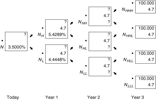
EXHIBIT 40–8
The One-Year Rates for Year 2 Using the Three-Year 4.7% On-the-Run Issue
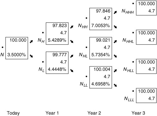
To verify that these are the correct one-year rates two years from now, work backwards from the four nodes at the right of the tree in Exhibit 40–8. For example, the value in the box at NHH is found by taking the value of $104.7 at the two nodes to its right and discounting at 7.0053%. The value is $97.846. Similarly, the value in the box at NHL is found by discounting $104.70 by 5.7354% and at NLL by discounting at 4.6958%.
USING THE LATTICE FOR VALUATION
To illustrate how to use the lattice for valuation purposes, consider a 6.5% option-free bond with four years remaining to maturity. Since this bond is option-free, it is not necessary to use the lattice model to value it. All that is necessary to obtain an arbitrage-free value for this bond is to discount the cash flows using the spot rates obtained from bootstrapping the yield curve shown in Exhibit 40–4. The spot rates are as follows:
1-year 3.5000%
2-years 4.2147%
3-years 4.7345%
4-years 5.2707%
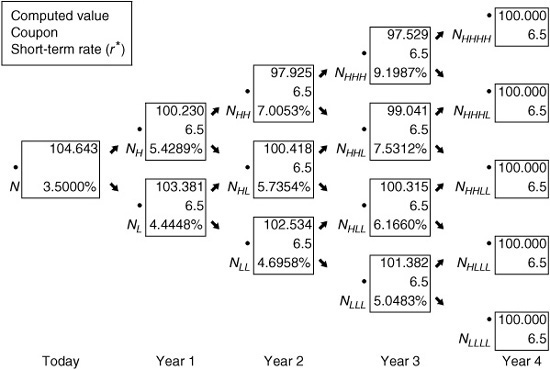
Discounting the 6.5% four-year option-free bond with a par value of $100 at the above spot rates would give a bond value of $104.643.
Exhibit 40–9 contains the fair tree for a four-year valuation. Exhibit 40–10 shows the various values in the discounting process using the lattice in Exhibit 40–9. The root of the tree shows the bond value of $104.643, the same value found by discounting at the spot rate. This demonstrates that the lattice model is consistent with the valuation of an option-free bond when using spot rates.
EXHIBIT 40–9
Binomial Interest Rate Tree for Valuing Up to a Four-Year Bond for Issuer (10% Volatility Assumed)
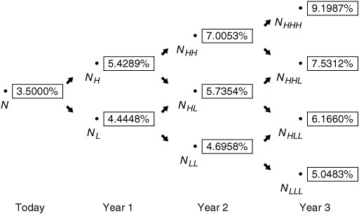
EXHIBIT 40–10
Valuing an Option-Free Bond with Four Years to Maturity and a Coupon Rate of 6.5% (10% Volatility Assumed)
FIXED-COUPON BONDS WITH EMBEDDED OPTIONS
The valuation of bonds with embedded options proceeds in the same fashion as in the case of an option-free bond. However, the added complexity of an embedded option requires an adjustment to the cash flows on the tree depending on the structure of the option. A decision on whether to call or put must be made at nodes on the tree where the option is eligible for exercise. Examples for both callable and putable bonds follow.
Valuing a Callable Bond
In the case of a call option, the call will be made when the present value (PV) of the future cash flows is greater than the call price at the node where the decision to exercise is being made. Effectively, the following calculation is made:
Vt = min[call price, PV(future cash flows)]
where Vt represents the PV of future cash flows at the node. This operation is performed at each node where the bond is eligible for call.
For example, consider a 6.5% bond with four years remaining to maturity that is callable in one year at $100. We will value this bond, as well as the other instruments in this chapter, using a binomial tree. Exhibit 40–9 is the binomial interest rate tree that was derived earlier in this chapter and then used to value an option-free bond. In constructing the binomial tree in Exhibit 40–9, it is assumed that interest rate volatility is 10%. This binomial tree will be used throughout this chapter.
Exhibit 40–11 shows that two values are now present at each node of the binomial tree. The discounting process explained earlier is used to calculate the first of the two values at each node. The second value is the value based on whether the issue will be called. Again, the issuer calls the issue if the PV of future cash flows exceeds the call price. This second value is incorporated into the subsequent calculations.
EXHIBIT 40–11
Valuing a Callable Bond with Four Years to Maturity, a Coupon Rate of 6.5%, and Callable after the First Year at 100 (10% Volatility Assumed)
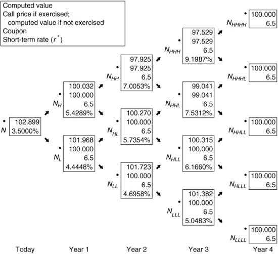
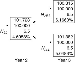
In Exhibits 40–12 and 40–13, certain nodes from Exhibit 40–11 are highlighted. Exhibit 40–12 shows nodes where the issue is not called (based on the simple call rule used in the illustration) in years 2 and 3.2 The values reported in this case are the same as in the valuation of an option-free bond. Exhibit 40–13 shows some nodes where the issue is called in years 2 and 3. Notice how the methodology changes the cash flows. In year 3, for example, at node NHLL the recursive valuation process produces a PV of 100.315. However, given the call rule, this issue would be called. Therefore, 100 is shown as the second value at the node, and it is this value that is then used as the valuation process continues. Taking the process to its end, the value for this callable bond is 102.899.
EXHIBIT 40–12
Highlighting Nodes in Years 2 and 3 for a Callable Bond: Nodes Where Call Option Is Not Exercised
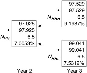
EXHIBIT 40–13
Highlighting Nodes in Years 2 and 3 for a Callable Bond: Selected Nodes Where the Call Option Is Exercised
The value of the call option is computed as the difference between the value of an optionless bond and the value of a callable bond. In our illustration, the value of the option-free bond is 104.643 (calculated earlier in this chapter). The value of the callable bond is 102.899. Hence the value of the call option is 1.744 (= 104.634 − 102.899).
Valuing a Putable Bond
A putable bond is one in which the bondholder has the right to force the issuer to pay off the bond prior to the maturity date. The analysis of the putable bond follows closely that of the callable bond. In the case of the putable, we must establish the rule by which the decision to put is made. The reasoning is similar to that for the callable bond. If the PV of the future cash flows is less than the put price (i.e., par), then the bond will be put. In equation form,
Vt = max[put price, PV(future cash flows)]
Exhibit 40–14 is analogous to Exhibit 40–3. It shows the binomial tree with the values based on whether or not the investor exercises the put option at each node. The bond is putable any time after the first year at par. The value of the bond is 105.327. Note that the value is greater than the value of the corresponding option-free bond.
EXHIBIT 40–14
Valuing a Putable Bond with Four Years to Maturity, a Coupon Rate of 6.5%, and Putable after the First Year at 100 (10% Volatility Assumed)
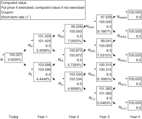
With the two values in hand, we can calculate the value of the put option. Since the value of the putable bond is 105.327 and the value of the corresponding option-free bond is 104.643, the value of the embedded put option purchased by the investor is effectively 0.684.
Suppose that a bond is both putable and callable. The procedure for valuing such a structure is to adjust the value at each node to reflect whether the issue would be put or called. Specifically, at each node there are two decisions about the exercising of an option that must be made. If it is called, the value at the node is replaced by the call price. The valuation procedure then continues using the call price at that node. If the call option is not exercised at a node, it must be determined whether or not the put option will be exercised. If it is exercised, then the put price is substituted at that node and is used in subsequent calculations.
VALUATION OF TWO MORE EXOTIC STRUCTURES
The lattice-based recursive valuation methodology is robust. To further support this claim, we address the valuation of two more exotic structures—the step-up callable note and the range floater.
Valuing a Step-Up Callable Note
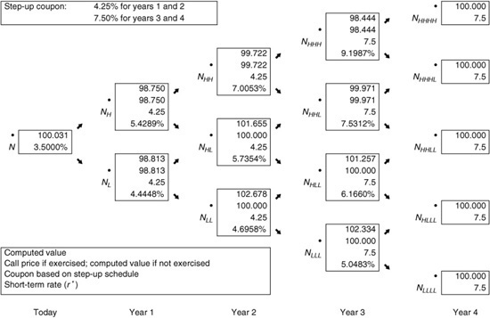
Step-up callable notes are callable instruments whose coupon rate is increased (i.e., “stepped up”) at designated times. When the coupon rate is increased only once over the security’s life, it is said to be a single step-up callable note. A multiple step-up callable note is a step-up callable note whose coupon is increased more than one time over the life of the security. Valuation using the lattice model is similar to that for valuing a callable bond described earlier except that the cash flows are altered at each node to reflect the coupon characteristics of a step-up note.
Suppose that a four-year step-up callable note pays 4.25% for two years and then 7.5% for two more years. Assume that this note is callable at par at the end of year 2 and year 3. We will use the binomial tree given in Exhibit 40–9 to value this note.
Exhibit 40–15 shows the value of the note if it were not callable. The valuation procedure is the now familiar recursive valuation from Exhibits 40–12 and 40–13. The coupon in the box at each node reflects the step-up terms. The value is 102.082. Exhibit 40–16 shows that the value of the single step-up callable note is 100.031. The value of the embedded call option is equal to the difference in the optionless step-up note value and the step-up callable note value, 2.051.
EXHIBIT 40–15
Valuing a Single Step-Up Noncallable Note with Four Years to Maturity (10% Volatility Assumed)
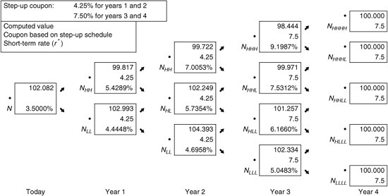
EXHIBIT 40–16
Valuing a Single Step-Up Callable Note with Four Years to Maturity, Callable in Two Years at 100 (10% Volatility Assumed)
Now we move to another structure where the coupon floats with a reference rate but is restricted. In this next case, a range is set in which the bond pays the reference rate when the rate falls within a specified range, but outside the range no coupon is paid.
Valuing a Range Note
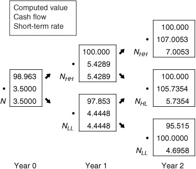
A range note is a security that pays the reference rate only if the rate falls within a band. If the reference rate falls outside the band, whether the lower or upper boundary, no coupon is paid. Typically, the band increases over time.
To illustrate, suppose that the reference rate is, again, the one-year rate and the note has three years to maturity. Suppose further that the band (or coupon schedule) is defined as in Exhibit 40–17. Exhibit 40–18 holds our tree and the cash flows expected at the end of each year. Either the one-year reference rate is paid, or nothing. In the case of this three-year note, there is only one state in which no coupon is paid. Using our recursive valuation method, we can work back through the tree to the current value, 98.963.
EXHIBIT 40–17
Coupon Schedule (Bands) for a Range Note
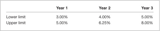
EXHIBIT 40–18
Valuation of a Three-Year Range Floater
EXTENSIONS
We next demonstrate how to compute the option-adjusted spread, effective duration, and the convexity for a fixed income instrument with an embedded option.
Option-Adjusted Spread
We have concerned ourselves with valuation to this point. However, financial market transactions determine the actual price for a fixed income instrument, not a series of calculations on an interest rate lattice. If markets are able to provide a meaningful price (usually a function of the liquidity of the market in which the instrument trades), this price can be translated into an alternative measure of value, the option-adjusted spread (OAS).
The OAS for a security is the fixed spread (usually measured in basis points) over the benchmark rates that equates the output from the valuation process with the actual market price of the security. For an optionless security, the calculation of OAS is a relatively simple, iterative process. The process is much more analytically challenging with the added complexity of optionality. And just as the value of the option is volatility-dependent, the OAS for a fixed income security with embedded options or an option-like interest-rate product is volatility-dependent.
Recall our illustration in Exhibit 40–11, where the value of a callable bond was calculated as 102.899. Suppose that we had information from the market that the price is actually 102.218. We need the OAS that equates the value from the lattice with the market price. Since the market price is lower than the valuation, the OAS is a positive spread to the rates in the exhibit, rates that we assume to be benchmark rates.
The solution in this case is 35 basis points, which is incorporated into Exhibit 40–19 that shows the value of the callable bond after adding 35 basis points to each rate. The simple binomial tree provides evidence of the complex calculation required to determine the OAS for a callable bond. In Exhibit 40–11, the bond is called at NHLL. However, once the tree is shifted 35 basis points in Exhibit 40–19, the PV of future cash flows at NHLL falls below the call price to 99.985, so the bond is not called at this node. Hence, as the lattice structure grows in size and complexity, the need for computer analytics becomes obvious.
EXHIBIT 40–19
Demonstration that the Option-Adjusted Spread Is 35 Basis Points for a 6.5% Callable Bond Selling at 102.218 (Assuming 10% Volatility)*

Effective Duration and Effective Convexity
Duration and convexity provide a measure of the interest rate risk inherent in a fixed income security. We rely on the lattice model to calculate the effective duration and effective convexity of a bond with an embedded option and other option-like securities. The formulas for these two risk measures are given below:
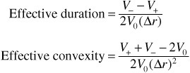
where V− and V+ are the values derived following a parallel shift in the yield curve down and up, respectively, by a fixed spread. The model adjusts for the changes in the value of the embedded call option that result from the shift in the curve in the calculation of V− and V+.
Note that the calculations must account for the OAS of the security. Below we provide the steps for the proper calculation of V+. The calculation for V– is analogous.
Step 1. Given the market price of the issue, calculate its OAS.
Step 2. Shift the on-the-run yield curve up by a small number of basis points (Δr).
Step 3. Construct a binomial interest-rate tree based on the new yield curve from step 2.
Step 4. Shift the binomial interest-rate tree by the OAS to obtain an “adjusted tree.” That is, the calculation of the effective duration and convexity assumes a constant OAS.
Step 5. Use the adjusted tree in step 4 to determine the value of the bond, V+.
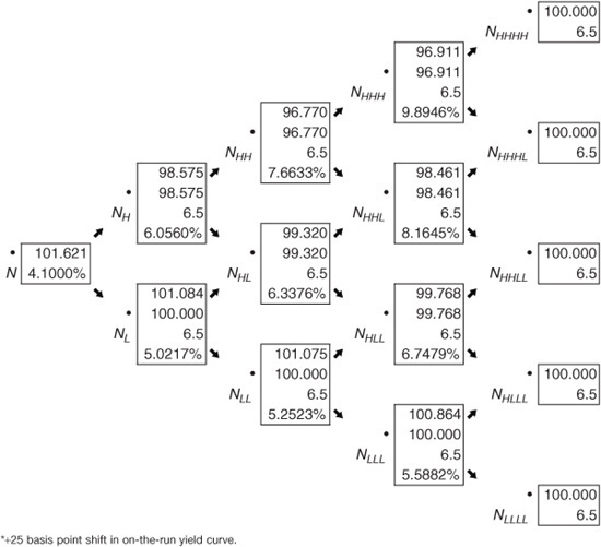
We can perform this calculation for our four-year callable bond with a coupon rate of 6.5%, callable at par selling at 102.218. We computed the OAS for this issue as 35 basis points. Exhibit 40–20 holds the adjusted tree following a shift in the yield curve up by 25 basis points and then adding 35 basis points (the OAS) across the tree. The adjusted tree is then used to value the bond. The resulting value V+ is 101.621.
EXHIBIT 40–20
Determination of V+ for Calculating Effective Duration and Convexity*
To determine the value of V−, the same five steps are followed except that in step 2, the on-the-run yield curve is shifted down by a small number of basis points (Δr). It can be demonstrated that for our callable bond, the value for V− is 102.765.
The results are summarized below:

Therefore,
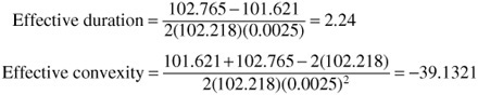
Notice that this callable bond exhibits negative convexity.
KEY POINTS
• For bonds with embedded options, the expected cash flow will depend on future interest-rate levels, which in turn depend on expected interest-rate volatility.
• An interest rate lattice provides a robust means for the valuation of a number of fixed income securities and derivatives.
• Given the market price of a bond, a lattice model can be used to obtain the option-adjusted spread to a benchmark yield curve based on an assumed interest rate volatility.
• A bond’s OAS is the fixed spread (usually measured in basis points) over the benchmark rates that equates the output from the valuation process with the actual market price of the security.
• Effective duration and convexity can be computed for a bond by changing the yield-curve up and down by a given number of basis points and calculating what the new prices would be on the revised interest rate tree. These new prices are then used in the standard duration and convexity formula.