CHAPTER
FIFTY
QUANTITATIVE MANAGEMENT OF BENCHMARKED PORTFOLIOS

LEV DYNKIN, PH.D.

Managing Director
Barclays Capital

JAY HYMAN, PH.D.

Managing Director
Barclays Capital

VADIM KONSTANTINOVSKY, CFA

Director
Barclays Capital

BRUCE D. PHELPS, PH.D., CFA

Managing Director
Barclays Capital

Most fixed income portfolios are managed relative to a benchmark. Depending on the portfolio’s investment objective and style, the role of the benchmark varies. At one end of the spectrum are passive indexed portfolios that strive to match benchmark risk exposures, and returns, as closely as possible. At the other end are active portfolios with high risk tolerance that maximize outperformance by investing freely outside the benchmark that serves only as a nonbinding reference point. The majority of fixed income portfolios fall somewhere between these extremes. Typically, a sponsor, an investment committee, a chief investment officer, or some other party that sets the investment objective specifies both the benchmark and the permissible deviations from it. The portfolio manager is then judged by the achieved outperformance versus the benchmark, and the amount of risk taken to generate this outperformance.

For the portfolio manager, the benchmark represents the zero-risk position. Over time, unless the manager deviates substantially from the benchmark, the portfolio’s absolute performance will be determined largely by the choice of the benchmark. Consequently, the choice of a portfolio’s benchmark is very important.

There is an ever-growing number of bond market indexes published by the leading investment banks and data providers. Often, an appropriate benchmark can be selected from this wide array of indexes. But there are many cases when none of the ready-made indexes serves the goals of the investor or plan sponsor. To ensure that the benchmark correctly reflects a given investment opportunity set and constraints, an existing index may need to be modified. Sometimes, a new, highly specialized index needs to be constructed. Finally, for some investors, the right benchmark may not even be a traditional total-return market index.

Fixed income markets are extremely diverse, so most indexes tend to include hundreds or thousands of securities. The sources of risk affecting fixed income securities are equally diverse and often difficult to analyze. These conditions turn even relatively straightforward portfolio tasks into complicated endeavors. For most portfolios, a seemingly trivial problem of “buying the benchmark” means selecting a relatively small subset of constituent securities while ensuring somehow that its behavior will be reasonably similar to the broad universe. Understanding portfolio risk versus a benchmark is equally complicated because of the many risk dimensions and intricate interactions among them.

As a result, essentially all functions of the bond portfolio management process are aided greatly by robust quantitative methods. This chapter reviews some major issues facing bond portfolio managers, as well as quantitative approaches for dealing with them: selecting and customizing a benchmark, analyzing portfolio risk and performance, replicating benchmarks, and optimizing portfolio structure to improve its risk-adjusted performance.

SELECTION AND CUSTOMIZATION OF BENCHMARKS

Financial literature lists several desirable qualities for performance benchmarks. A good benchmark is investable, transparent, known in advance, and diversified. However, it is not always possible to achieve all of these goals. While these are all important attributes, first and foremost, the benchmark should be appropriate. An appropriate benchmark matches the required strategic allocation of portfolio assets, so that the portfolio’s performance will be broadly consistent with the investor’s overall objectives. A benchmark should also be investable so that a manager can “buy the benchmark” if and when he so decides. When comparing portfolio performance to the benchmark, it is critical to know when any difference owes to the manager’s decisions and not to any in-built mismatches beyond the manager’s control. Any constraints that limit the portfolio opportunity set must be reflected in the benchmark as well.

An index may provide an accurate gauge of the performance of a particular segment of the fixed income markets, but that does not necessarily make it an appropriate benchmark. For example, while the Barclays Capital U.S. Aggregate Index is a widely used benchmark for the U.S. investment-grade fixed income market, the average duration of this index (4.59 as of 10/31/10) may make it unsuitable for portfolios funding long-duration liabilities.

Reflecting Investor Opportunity Set and Constraints

When an investment policy requires specific allocations to certain asset classes or imposes other restrictions such as a duration target, a customized index may be a more appropriate benchmark. In the simplest case, a customized index merely changes relative weights of standard components while still including all securities in the standard index. Often, investment policy may impose a minimum credit-rating threshold on the securities that the portfolio can buy. Limitations may be placed on maximum exposure to an industry, country, and so on. Many other bond attributes, such as minimum or maximum maturity, age, coupon, etc., may also be controlled, requiring corresponding changes to the benchmark. In all cases, though, the goal should be to keep the benchmark as broad-based and well-diversified as possible while still meeting all the investment policy requirements. However numerous the modifications to the original market-based index, one important benchmark property always should be preserved: objectivity. The benchmark should be based on a set of rules specified beforehand and kept constant. The rule-based nature of a benchmark also allows for a historical analysis of its past behavior. Such analysis can be quite useful at the stage of selecting a benchmark.

One widely used method to achieve outperformance is to invest outside the benchmark. Such investments (e.g., high-yield credit or emerging market debt) frequently are referred to as “core-plus.” Even when the exposure to core-plus assets is constantly present in the portfolio, many managers still prefer to keep such assets out of the benchmark. Their motivation, of course, is to keep this potential source of outperformance at their disposal. However, a case can be made for inclusion of frequently used core-plus assets into the benchmark. First, by including these assets in the benchmark, the manager’s relative performance will be more fairly measured if the manager has a persistent allocation to these assets. Second, it is often difficult to “short-sell” core-plus type assets. Yet a manager who has expertise in these markets can benefit from a short position just as much and as frequently as from a long position. The only way to effectively short such assets is to underweight them versus the benchmark. This, of course, is only possible when they are included in the benchmark. Such a benchmark decision should be made only after ensuring that with the inclusion of these asset classes, the benchmark will remain appropriate for the portfolio’s investment objective and style.

Targeting Duration/Cash-Flow Profile

Sometimes a customized benchmark is necessary not because of sector, quality, or other allocation constraints but because the portfolio is expected to have a particular term-structure exposure. For example, some portfolios are managed to provide a particular cash-flow stream to fund a set of liabilities. At the simplest level, portfolio duration may be kept equal to the duration of the liability stream. Dedication is another widely used method for ensuring the necessary cash-flows while (usually) minimizing the portfolio cost. Of course, funding the future liabilities is the main investment objective in such cases. Yet investment policies of liability funding portfolios can be quite liberal, providing an opportunity for outperformance while still ensuring sufficient cash flows.

Such portfolios would benefit from a diversified benchmark with a cash-flow profile that matches the expected liability stream and at the same time fully reflects the manager’s opportunity set. Consider, for example, a liability funding portfolio that is free to invest in any security in a credit index. An appropriate benchmark for such a portfolio could match the sector and quality distribution of the index while also matching the cash-flow profile of the liabilities. Such a “liability-based” benchmark retains many of the desirable attributes of a broad market-based index: it is objectively-defined, so the portfolio manager can stay neutral to it, and its returns are calculated using market prices. Because this benchmark consists of marketable securities, its performance can be calculated and published by a third-party index provider.¹

Even outside the asset/liability context, many fixed income portfolios are managed with a specific duration target. If this target is not close to the duration of any standard (published) index, an appropriate benchmark may be constructed as a blend of two published indexes, one of which is longer and the other shorter than the target. Although the weights needed to achieve a desired duration may have to be adjusted at regular intervals, they typically remain fairly stable for indexes that consist mainly of option-free securities.

Things get more complicated for portfolios containing a large proportion of securities with embedded optionality. Duration of such portfolios is likely to be unstable, changing in response to interest-rate movements. For example, the duration of mortgage-backed securities (MBS) can be quite volatile. If maintaining a stable duration is an important requirement, managers may engage in such techniques as delta hedging to overcome the effect of negative convexity and keep duration relatively constant. Hedging techniques entail various costs, from the more obvious transaction costs to the less obvious but potentially more significant “whipsaw” costs.² It is unfair to judge the performance of a manager who must engage in costly delta hedging against a benchmark that does not bear similar costs. Two possible solutions are: to apply delta hedging to the benchmark; or to construct a “constant duration” index that provides a fairer benchmark for a delta-hedged mortgage portfolio.³ An example of such a benchmark could be a market-weighted MBS index dynamically hedged, according to a set of rules, with a liquid leveraged overlay of Treasuries or futures contracts.

Asset-Swapped Indexes

Some investors can take credit positions but are required to match the interest rate exposure to their funding source (e.g., three-month LIBOR). For example, some bank and insurance investment managers must manage their portfolios to a short duration target for asset/liability management purposes but are free to exercise their credit skills in asset selection. Leveraged investors often concentrate on credit exposure but minimize interest-rate exposure by managing the portfolio duration to the short-term LIBOR funding. In an environment of moderate credit-spreads and low interest rates (and worries about rising rates), traditional total return managers are also likely to keep durations very short while maintaining an overweight to spread sectors. These managers want to exercise their credit skills but avoid term-structure risk.

The most straightforward way to create and maintain such exposures is to turn to the floating-rate note market. However, given limited issuance, this may create an unintended concentration of systematic sector exposures or issuer idiosyncratic risk. Ideally, the manager would want to match systematic spread-sector risks (i.e., credit quality and sector exposures) of a broad credit market index while simultaneously removing exposure to all systematic Treasury key-rate risk factors except, perhaps, the shortest (e.g., three or six-month) key rate. The challenge of designing a benchmark for such a portfolio is to ensure a very short Treasury duration and at the same time match the overall index allocations to the credit sectors.

To exercise their spread-sector timing skills while minimizing interest-rate exposure, investors can buy fixed-rate spread assets on an “asset-swapped” basis. Asset swaps are combinations of a fixed-rate bond (and its credit exposures) and an interest-rate swap that exchanges the fixed-rate coupons for floating-rate coupons. An asset swap gives an investor an opportunity to take spread-sector exposure with little term-structure risk.

There are no formal indexes of asset swap performance. To benchmark an asset-swapped portfolio effectively, the benchmark must represent a “neutral” spread-sector allocation. Then the manager’s deviations from neutral may lead to outperformance of the benchmark. Using three-month LIBOR as a benchmark is inadequate because LIBOR reflects only a single type of spread risk (i.e., swap spreads) and does not represent the wide array of spread-sector choices that may be available to the manager. An ideal design for asset-swapped portfolios is a floating-rate benchmark that reflects a diversified set of spread-sector exposures. One approach to constructing such benchmarks⁴ starts with the creation, for each asset class, of a “mirror” swap index, which is a portfolio of interest rate swaps that has the same key-rate duration profile as that of the “mirrored” asset class. Then, short positions in these mirror-swap indexes are combined with long positions in the corresponding asset-class indexes, as well as with a long position in a short-term asset (e.g., one-month LIBOR). This creates “asset-swapped indexes” for all asset classes in the benchmark. Finally, individual asset-swapped indexes are merged into the final composite benchmark according to the portfolio’s “neutral” allocations.

Book Accounting Based Indexes

Fixed income investors typically measure portfolio performance by calculating returns using market prices at the beginning and end of the performance period. Consequently, the portfolio’s market value fluctuates with changing Treasury yields, spreads, and prepayments. Most standard fixed income indexes are market-return based, and many analytical tools make the same assumption about portfolios.

However, there is a large class of investors (e.g., insurance companies and banks) less concerned about short-term market fluctuations. They purchase fixed income assets to match a set of liabilities whose net present value is based not on market prices, but on book, or purchase, prices. Typically, these fixed income portfolios are relatively static. Investors expect the portfolio to earn an adequate spread over the cost of the liabilities, assuming that the assets do not default or prepay at a rate unanticipated at the time of purchase. Given that liabilities are valued using book accounting, these investors (and their regulators) need to measure asset portfolio performance similarly either by the portfolio’s “book return,” which is book income divided by book value, or the portfolio’s “book yield,” which is its internal rate of return calculated at time of purchase. However, how can such investors measure their investment skill when most indexes are market-return based?

Book accounting based investors can measure their performance relative to book accounting based indexes, or “BOOKINs,” that are, in theory, replicable investment portfolios. For example, suppose that in January 2011, an investor restricted to assets in the Barclays Capital Aggregate Index must fund a newly acquired liability. The investor could passively invest in the January 2011 Aggregate BOOKIN. The composition of this BOOKIN is set to reflect the Aggregate Index as of January 2011, and its book yield and book return are calculated every month. Over the course of the month, the BOOKIN will generate cash-flow (coupon, prepayments, proceeds from maturities), which is reinvested in the February 2011 Aggregate Index. Consequently, by February 2011, the JAN11 Aggregate BOOKIN becomes a conglomeration of the initial investment in the January Aggregate Index plus a smaller investment in the February Aggregate Index. This process is repeated every month. The performance of the JAN11 Aggregate BOOKIN, expressed in book accounting terms, reflects what the investor could have achieved by passively investing in the Aggregate Index starting in January 2011, and thus can be directly compared with the book accounting performance of the investor’s actual portfolio.⁵

Strategy-Based Indexes

Finally, some portfolio managers must operate under severe performance constraints such as “over the next three months generate as much return as you can, but don’t lose any money!” Many official institutions manage their Treasury portfolios under such constraints. What is an appropriate benchmark for these investors? While a cash benchmark (i.e., zero duration) would not suffer any losses, it would severely limit income. In contrast, a longer duration benchmark would likely generate more income but put the portfolio at risk of losses over the holding period.

The right benchmark would have a duration that maximizes expected returns subject to the risk constraint. But, how to best generate expected returns to determine the benchmark? Using historical Treasury returns data is one approach. An advantage of historical returns is that they are non-subjective estimates of expected returns. However, historical returns are poor predictors of future returns. Another approach is to use expected returns embedded in the current term structure. These estimates are also non-subjective (i.e., “no-view”) because they assume only that the yield-curve will remain unchanged. These no-view expectations reflect current market conditions whereas historical returns do not.

A benchmark can be constructed using no-view expected returns and historical volatilities to maximize expected return subject to a risk constraint of not having a return less than zero with a pre-specified probability. The solution to this optimization problem is a Treasury portfolio that would serve as the benchmark. The manager would then be responsible for outperforming it. Alternatively, the manager could simply hold the benchmark if he did not wish to take any risk. This “no-view” Treasury benchmark is an example of how benchmarks can be objectively designed to reflect investment goals and constraints.⁶

DIVERSIFICATION ISSUES IN BENCHMARKS

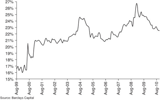
Issuer-specific risk is an important consideration in credit portfolios. Increasingly, though, benchmarks are also scrutinized for any embedded security-specific risks. Excessive exposure to individual issuers is a concern not just for portfolio managers. Plan sponsors now reexamine benchmark design and pay close attention to large issuer concentrations. This is a serious issue even for the users of very broad market indexes. As Exhibit 50–1 shows, as of October 2010, the top 10 issuers in the Barclays Capital U.S. Corporate Bond Index accounted for 23% of the overall market value. For some plan sponsors, this is too much security-specific risk. An asset manager benchmarked to this index may feel compelled to have exposure to some of these large-cap issuers because they have significant weights in the benchmark. Concerns about the high level of issuer concentration risk in some commonly adopted benchmarks led to a number of developments in benchmark design that attempt to mitigate this risk.

EXHIBIT 50–1
Market Value Weight of the Top Ten Issuers in the Barclays Capital U.S. Corporate Bond Index, August 1999–October 2010

Issuer-Capped Benchmarks

A cap on the market-value weight that an issuer can have in the index limits exposure to the issuer’s idiosyncratic risk. When such a cap (e.g., 1%) is imposed, every issuer’s capitalization is checked against this ceiling. The market value in excess of the cap is “shaved off” and then distributed to all other issuers in the index in proportion to their market-value weights. Different caps can be chosen for various credit ratings, reflecting the differences in issuer-specific risk between higher and lower credit qualities. While issuer-capped portfolios have existed for quite a while, issuer-capped benchmarks are more recent and emerged in response to the increased levels of issuer-specific risk in credit markets.

Issuer-capped indexes seem very straightforward. However, the cap level and the redistribution rule can have a significant impact on the risk and return characteristics of an index. Some redistribution rules can limit the benefits of issuer capping by inadvertently introducing unfavorable sector-quality risk exposures relative to the uncapped index.⁷

For example, an “index-wide” redistribution rule allocates the “excess” market value across all non-capped issuers in the index in proportion to their weights. However, this may produce an index with very different (and most likely unintentional) sector and quality exposures compared with the uncapped index. For example, the following table covering the period August 1989 through October 2010 shows that the index-wide redistribution rule in a 1% issuer-capped Barclays Capital U.S. Corporate Bond Index produces significant overweights in Baa-rated and industrial issues and a significant underweight to financials compared with the uncapped Corporate Index:

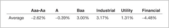
This inadvertent introduction of potentially unfavorable sector-quality risk exposures can be avoided by a “quality-sector-neutral” redistribution rule that preserves the sector and quality profiles of the uncapped index.

Another side effect of capping large issuers in an index is the increase in weights of smaller ones. By construction, in a capped index the market-value weights of smaller issuers exceed their actual weights in the marketplace, sometimes dramatically so. This raises a practical concern that the available market supply may not allow the manager to match (if he or she so chooses) the required allocation in the issuer-capped index.

Issuer-capping has also been applied to sovereign indexes. The distribution of sovereign issuers is highly concentrated. For example, based on market value weights, Japan represents almost 32% of the Barclays Capital Global Treasury Index (as of 12/31/2010), and the U.S. almost 26%. Together, Japan and the U.S. comprise almost 60% of the Global Treasury Index. Within geographical regions these country weights are even larger, as Japan Treasuries account for over 90% of Asian Treasury bonds while U.S. Treasuries account for 92% of Treasuries in the Americas. The skewed distribution of sovereign issuers may make issuer-capping attractive to investors. However, as with issuer-capped credit indexes, care must be exercised when redistributing any excess capped market value.

A simple sovereign capping scheme of redistributing any excess market value above a cap level across all smaller sovereign issuers in the index does little to reduce the volatility of the index. This is because the excess capped market value gets proportionally reallocated to other countries that are closely related economically to the capped countries. A more productive sovereign capping scheme is first to cap the market value weight of economic regions, and redistribute excess market value across other regions. Then, cap individual sovereigns within a region and redistribute any excess capped market value within the region. Such a two-tier capping scheme reduces the volatility of the index, compared to the uncapped sovereign index, and does not hurt the index’s performance.

An alternative sovereign capping scheme is to adjust index market value weights depending on the relative economic fundamentals across countries. For example, countries whose Debt/GDP levels are below average would have their index market value weights increased, while those countries with above average debt levels would have their weights lowered.⁸ Such “fundamental-based” weighting schemes have become more popular as sovereign creditworthiness has become less certain.

Despite these subtle issues, issuer-capped indexes are now a permanent fixture of the investment management landscape. With good judgment, investors can design issuer-capped indexes that meet their risk-management preferences in dealing with issuer-specific risk.

Swap-Based Benchmarks

A somewhat radical approach to dealing with issuer-specific risk in credit benchmarks is not to have this risk at all. Apart from the naive solution of adopting an all-Treasury benchmark, one popular type of benchmark is based on interest-rate swaps. Swaps offer excellent liquidity, a virtually unlimited market supply, limited idiosyncratic or “headline” risk, and an opportunity to capture some of the long-term spread advantage of investing in non-Treasury product. Swaps have been a key feature of the debt markets since the early 1990s. In fact, in several ways the swaps market is larger and more heavily traded than the U.S. Treasury market.

Swap payments are based on LIBOR, and therefore, the par swap rate curve can be viewed as a generic yield-curve for large, highly rated banks whose interbank lending rates constitute the LIBOR index.⁹ Correspondingly, the swap spread (to the Treasury curve) is considered a generic proxy for high-grade credit spreads. (While the swap spread does not reflect counterparty risk, this can be effectively eliminated through collateral management.)

This relationship between interest rate swap spreads and high-grade credit-spreads has prompted some investors to consider swaps as total return benchmarks for their credit portfolios. However, unlike returns on regular fixed income securities, returns on swaps are not directly observable in the marketplace. In addition, while cash fixed income securities have an underlying market value that serves as the base on which to calculate returns, par swaps at initiation have zero market value. While swap yields and spreads are available from many sources, swap returns are not. To create total return indexes for the swaps market, a new index methodology is needed.

The Barclays Capital interest rate swap index methodology¹⁰ relies on the creation of hypothetical constant-maturity swap “securities” from the swap curve. At the start of every month a set of par receive-fixed swaps is identified with swap rates taken from the specific maturity points on the swap curve. To create, say, the 10-year swap index the 10-year par swap is paired with a cash investment in three-month LIBOR equal to the notional amount of the swap. Over the course of the month, the mark-to-market return of the 10-year swap is combined with the mark-to-market of the LIBOR deposit, divided by the initial notional value, to produce a 10-year swap index return. There are as many swap indexes as there are maturity points on the swap curve. There are interest rate swap indexes not only for USD, but for other currencies as well (e.g., EUR, GBP, and JPY).¹¹

The individual swap indexes can be combined to produce a swap index with any desired term-structure profile (e.g., to match a particular liability duration target). Recall the earlier discussion on asset-swapped benchmarks where each asset class had an associated swap index (the mirror swap index) with a matched key-rate duration profile. A credit portfolio manager who has a swap index as a benchmark is completely free to hold only those credits which he thinks will outperform and to avoid credits expected to underperform duration-matched swaps. Credits on which the manager is neutral or has no view need not be in the portfolio at all. In contrast, if the manager’s benchmark is a market index, he is under pressure to have at least some exposure to the largest issuers in the benchmark. Even when the manager has a negative view on a large issuer in the corporate index, he is unlikely to hold a zero weight because that creates a large active bet against the benchmark.

Downgrade-Tolerant Benchmarks

Even in periods of severe spread volatility, many investors retain a persistent allocation to credit in the belief that given sufficiently long time, credit bonds earn a meaningful spread premium over comparable duration Treasuries. Credit-spread premium refers to any excess return net of realized default losses, not including the impact of spread changes. A buy-and-hold credit investor earns the spread premium to maturity and ignores mark-to-market volatility in the interim.

But do investors indeed capture this credit-spread premium? In theory, they do, as long as they maintain a hold-to-maturity allocation to credit. In reality, however, most investors use a market benchmark to represent their credit allocation. In the case of Barclays Capital investment-grade indexes, for example, the index rules stipulate that a bond downgraded below investment grade be dropped from the index. Accordingly, portfolios benchmarked to the index have to sell these bonds. Usually, this is precisely when the spreads of such bonds are particularly wide, often wider than justified by any subsequent default losses. This bad timing may cause index-benchmarked investors to forfeit, at least partially, the credit-spread premium.

An alternative is to allow managers to hold on to downgraded bonds and choose their own timing in selling such bonds.¹² Such a “downgrade-tolerant” Corporate Index has captured a spread premium almost 80% higher than the standard index. Exhibit 50–2 plots a yearly comparison between the two, for the period from 1990 through 2009. The downgrade-tolerant index delivers a higher premium in every one of these 20 years, with virtually the same risk profile as the standard index.¹³

EXHIBIT 50–2
Estimated Annual Credit-Spread Premium, 1990–2009, % per Year

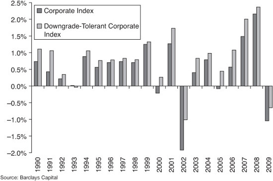
These results suggest that if managers are allowed to hold on to bonds that the Corporate Index discards, they should be able to harvest a considerably higher spread premium and significantly improve their performance versus the benchmark.

PORTFOLIO ANALYSIS RELATIVE TO A BENCHMARK

The selection of the investment guidelines and appropriate benchmark marks the beginning of the portfolio management process. Once a portfolio is established, investors continually monitor its positioning relative to the benchmark. Apart from investing new funds, periodic transactions help to maintain desired exposures and express changes in market outlook.

Certain portfolio monitoring activities are typically performed at regular intervals (say, a calendar month) and in a set sequence. Other analyses are performed as the need arises and not necessarily in a fixed order. Yet, however different the operational details might be, there are certain common functions that portfolio managers must perform and certain types of tools necessary to carry out these duties. Typically, at the start of a performance period, managers will use forward-looking, or ex-ante, analytics to create and ascertain the desired portfolio positioning. At the end of the period, managers will use backward-looking, or ex-post, analysis to review and explain the realized performance which, in turn, guides portfolio adjustments.

Analyzing Portfolio Risk: A Cell-Based Approach

The most obvious way to analyze portfolio-versus-benchmark risk is a structural comparison of the two by partitioning them into a matrix of cells. Different choices of partition variables put the focus on different aspects of portfolio composition. Corporate portfolios, for example, are likely to be divided by quality and industry category (e.g., basic industry, consumer cyclical, and energy). Segmenting by duration highlights the yield-curve exposure. The amount and quality of information a portfolio manager can derive from such reports depend on the appropriateness of the chosen risk dimensions and on the portfolio and benchmark attributes (beyond market-value percentages) available for comparison.

The fundamental assumption behind the use of structural reports is, of course, that the contribution of a mismatch in a given cell to the overall portfolio-versus-benchmark risk is primarily a function of the magnitude of the mismatch and the weight of the cell. This assumption is not unreasonable. Certainly, a portfolio that matches its benchmark in all cells (along all possible dimensions) is risk-neutral to the benchmark.

While the simplicity of such analysis is attractive, there are two major problems with its basic assumption. First, the risk consequences of a particular mismatch depend not only on its apparent magnitude but also on its nature, i.e., the volatility of the underlying exposure. A mismatch in spread duration contribution of 1.0 in Aa financials has a very different risk than the same-size mismatch in Baa telecom. Granted, some experienced portfolio managers may have a feel for the portfolio performance implications from the magnitudes of individual mismatches.

However, the second problem is equally important and, arguably, more difficult to compensate for with experience. The cross-correlation among the multiple sources of risk in a portfolio makes judging overall risk a daunting one without quantitative tools. Two mismatches in two different cells, each entailing significant risk in isolation, may cancel each other if low (or even negative) correlation between them reduces their joint contribution to risk. Conversely, a few mismatches that could easily be ignored individually may represent a serious risk if the correlations among them are high. Needless to say, when the number of mismatches reaches dozens, as it can even in relatively simple portfolios, finding the common risk denominator by “eyeballing” the structural mismatches is unrealistic.

Analyzing Portfolio Risk: Multifactor Risk Models

One reliable approach to quantifying a portfolio’s active risk (i.e., risk versus benchmark) is multifactor risk analysis. Its primary goal is to help managers to structure portfolios with desired risk exposures relative to the benchmark. As such, it is generally used not as an ex-post control tool but rather as an ex-ante tool for portfolio structuring. One obvious need is to measure the expected risk of return deviation in portfolios that track a benchmark. Another is to form a reliable estimate of risk for active managers with a particular outperformance, or “alpha,” target. There is a well-established consensus among investment professionals regarding realistic levels of information ratio, or risk-adjusted outperformance, versus the benchmark. A realized information ratio above 0.5 generally is considered to be quite high, with 1.0 often seen as a practical upper limit. As a result, quantifying active risk allows managers to test the feasibility of a specified alpha target. For example, a portfolio with an alpha target of 50 basis points per year should be allowed an active risk somewhere in the range of 50 to 100 basis points per year. If, as a result of policy constraints, the projected risk is estimated to be much lower, the manager should make a case for either relaxing portfolio constraints or revising downward the alpha target.

Active risk has systematic and idiosyncratic components. The former is a result of the differences between the portfolio and benchmark sensitivities to common market risk factors (e.g., movements of the key rates, credit sector spreads, or volatility). The latter, sometimes referred to as “diversifiable risk,” reflects unequal exposures (usually overweights in the portfolio) to individual issuers and can be present even when all systematic exposures are eliminated. This type of risk reflects residual spread movements of individual issuers, not explained by anything that happens to their peer group. Apart from the risk of typical idiosyncratic spread movements, there is default risk which is particularly important in lower-quality credit portfolios. For example, in the Barclays Capital risk model, default risk is modeled and reported separately from market risk. Conceptually, default risk contains both systematic and idiosyncratic parts. Correlated defaults across different issuers create a systematic risk component. To the extent that defaults are uncorrelated and reflect unusual events specific only to a particular issuer, the default risk is idiosyncratic risk. Separating the systematic and idiosyncratic components of default risk is quite difficult.

To quantify the systematic component of market risk, multifactor risk models use historical volatilities and correlations of a relatively small set of risk factors. These are processed into a covariance matrix that is the cornerstone of the model. The idiosyncratic component of active risk is quantified by measuring the differences between the portfolio and benchmark concentrations in a specific issue or issuer. These weight differentials are then multiplied by idiosyncratic spread volatilities specific to a given issuer or its peer group.

These risk components are combined to produce the key output of such models—tracking-error volatility (TEV), defined as the projected standard deviation of the monthly return differential between the portfolio and the benchmark. TEV is an extremely useful measure because it provides a common unit for many different sources of risk, enhancing comparisons of diverse exposures and greatly facilitating portfolio risk management and risk budgeting. Well-developed models not only compute TEV but also provide useful information on its components, for example, detailed analysis of the TEV sources, their relative contribution to the total, and their interdependence.¹⁴

Of course, the reliance on historical observations exposes the multifactor analysis to criticism that risk-factor correlations are unstable and depend (as do volatilities) on the economic cycle. These concerns, however, are easily addressed.

Different historical periods can be viewed as more or less relevant to the current environment. Some asset classes evolve over time, and their risk characteristics change. For example, the dramatically increased refinancing efficiency in the U.S. residential mortgage market made MBS prepayment history up to the early 1990s largely irrelevant for estimating prepayment risk in subsequent periods. Economic and market conditions also may justify emphasizing a particular historical period while downplaying others. Risk models can accommodate these risk dynamics. One mechanism is to impose time decay on the historical data series to give greater weight to more recent data.

The idiosyncratic component of active risk presents a bigger challenge to history-based risk models. To quantify the issuer-specific risk, a model needs estimates of residual spread volatility in all market segments. These estimates can be derived only from the historical time series of individual securities’ residual returns; that is, parts of each bond’s return unexplained by all the systematic risk factors. This requires a large body of individual security-level historical data.

As with systematic risk, there is the issue of choosing a relevant historical period for the idiosyncratic risk estimation. Conservatism is usually a good rule of thumb. After a spike in issuer-specific volatility, such as the one that happened in the U.S. credit market in 2008, a risk model needs to “learn” quickly from recent experience. Applying time decay to the historical data accomplishes this and makes the model produce higher estimates of idiosyncratic risk going forward. Sometimes, however, a risk model should pay less attention to recent experience. After a long period of calm, the model should revert to the equal weighting of historical data to avoid underestimating issuer risk.

History-Based Scenario Analysis

In one form or another, scenario analysis is used widely by portfolio managers to study portfolio (and benchmark) behavior in various yield-curve, spread, volatility, prepayment, or exchange-rate environments. Managers focus on what they consider the most likely scenarios, or unlikely but potentially damaging scenarios. Scenario analysis complements multifactor risk analysis. It allows managers to stress-test benchmarked portfolios by subjecting them to extreme conditions (“three-standard-deviation events”) not necessarily consistent with the history underlying the risk model. Such analysis may highlight potential sources of return deviations that do not manifest themselves under normal (by historical standards) circumstances.

When using scenario analysis, investors usually make explicit forecasts for specific, observable market dimensions: key interest rates, credit-spreads for certain market sectors, particular exchange rates, and such. It is very difficult, however, to formulate scenarios that are consistent in both direction and magnitude across many different market sectors and to estimate the probability of such scenarios. This is similar to analyzing risk simultaneously along many dimensions. Thus the solution also can be the same as in multifactor risk models. A covariance matrix estimated from historical observations can be used to build “maximum-likelihood scenarios.” Such scenarios incorporate a few explicit forecasts provided by the investor and then infer historically-consistent realizations (forecasts) for all other factors in the matrix. Then the full set of stated and derived factor forecasts is translated into expected returns for individual securities.

Explicit forecasts may represent unlikely scenarios. For example, the projection of a one-month yield increase of 50 basis points (or more) represents a 2.3% probability event if the historical yield volatility is only 25 basis points per month (assuming a normal distribution). Similarly, historical correlation patterns would not support an expectation of credit-spread widening at the same time with an increase in Treasury yields because yield and spread changes typically are negatively correlated. A scenario-generation model can be made to assess the likelihood of an explicit forecast in light of the covariances that underlie the analysis and to allow a rescaling of forecasts to meet pre-specified likelihood targets. The views can be relative as well as absolute. A yield-curve slope forecast is an example of a relative forecast because it does not express an opinion on the overall direction of interest rates. Individual forecasts can be accompanied by degrees of confidence in them. For example, investors usually are more confident in their views on credit-spread movements than on currency and interest-rate changes. A robust scenario analysis framework should be able to incorporate this information.

Attribution of Portfolio Performance Relative to a Benchmark

A comprehensive performance-attribution framework must account for all potential sources of portfolio performance and quantify the contribution from each of these sources. Performance attribution of past returns is perhaps the most important tool that asset managers can use to substantiate their claims on expertise in a given style of investment. If, for example, an investment fund claims to be adept at finding undervalued credits, performance attribution can be used to determine what share of the fund’s past outperformance was due to credit picks. Unless there is hard proof that the generated returns came from the advertised source, investors may worry that superior performance might have been luck rather than skill and may, in fact, be a sign of imprudent risk taking.

Asset management companies also benefit from using performance attribution in the internal analysis to help determine their skill in managing different kinds of exposures and the areas that need improvement. Sources of achieved outperformance should be matched with sources of ex-ante risk. Quantitative analysis of return deviations from the benchmark may point out unintended portfolio exposures that need to be corrected. This is particularly important for large funds with decentralized decision making in which separate groups or individuals are responsible for yield-curve positioning, sector and quality allocations, and name selection. Performance attribution can help evaluate individual manager performance in such an organization. Flexibility is critical in this analysis. A performance-attribution framework will only be useful (and used) if it is aligned with the actual decision-making process behind the portfolio investments. This process differs across firms and may vary over time within a single firm.

For multicurrency portfolios, the analysis normally starts at the global level, where outperformance can be traced to two basic sources: exchange-rate exposures and asset allocation exposures to different markets. The ability to implement currency hedges as an overlay using FX futures or forwards empowers managers to separate the asset allocation and currency allocation decisions. The attribution framework should explain the performance due to each.

After multicurrency outperformance is assessed, portfolio positions generally should be segregated by currency, and the performance of each single-currency portfolio evaluated separately (versus appropriate single-currency benchmarks). In a developed fixed income market, such as the United States, local returns can be divided into three main components: Treasury (yield-curve), volatility, and spread.

The Barclays Capital performance-attribution system relies on the key-rate duration¹⁵ methodology to compute outperformance owing to the Treasury curve positioning. Both the portfolio and the benchmark are replaced by hypothetical portfolios of Treasuries with exactly the same yield-curve exposures, that is, with matching key-rate duration profiles. Then the returns of these “Treasury-matched” portfolios are compared. Any difference comes exclusively from their disparate curve exposures. The bonds in the Treasury-matched portfolios usually are not real securities but rather points from the par yield-curve, and contribute no pricing noise (such as owing to the richness of on-the-run issues). The model breaks down this component of outperformance even further to individual key-rate exposures.

A shift in implied volatility affects prices of bonds with embedded optionality. Quantifying outperformance owing to differences in volatility exposure requires a good term-structure model that can estimate the implied volatility of the Treasury curve and the analytics to compute volatility sensitivity (or vega) for all securities in the portfolio and in the benchmark.

Outperformance owing to spread exposure can be broken into an asset allocation part (asset class, sector, industry, quality, etc.) and a security-selection part. The former occurs when the portfolio had larger allocations to winning asset classes (or smaller to losing) than the benchmark. Security-selection outperformance comes from picking names that outperform their peers. Both measures depend strongly on the definition of asset classes or security peer groups.

Performance attribution is one of the most complex elements in a suite of methodologies and tools that modern asset managers need. There are many technical points and subtleties, such as aggregating daily results, accounting for intraday trading, and dealing with pricing and return conventions that differ between the portfolio and the benchmark.

QUANTITATIVE APPROACHES TO BENCHMARK REPLICATION

Besides index funds whose investment mandates explicitly call for tracking benchmarks with the minimum possible deviation, “buying the benchmark” is often a reasonable tactic even for managers who normally pursue active strategies. For example, in times when managers have no definite views on particular segments of the market, matching index returns in those segments is a sensible strategy. Sometimes, when managers have accrued significant outperformance before the year is over, they decide to switch to passive benchmarking for the rest of the year to preserve their gains. Finally, investors sometimes use so-called proxy portfolios that replicate broad market indexes for modeling purposes rather than for direct investment. The main reason usually is to apply the same in-house models (e.g., prepayment models) to both the portfolio and the benchmark, eliminating “model noise” that can be quite significant. Sometimes it is not feasible to include the actual benchmark in the analysis because of constraints on either processing time or data availability. Computer-based analysis gets simpler and faster when applied to a small set of well-priced securities as opposed to potentially thousands of bonds in an index. Hence, the term proxy portfolios.

As pointed out earlier, the replication of a diverse market index that has multiple sources of return is not a trivial task and requires complicated techniques and tools. There are two main techniques: replication with actual, or “cash,” securities and replication with derivative instruments (e.g., futures and swaps). The replication strategies vary greatly, reflecting diverse characteristics of various fixed income markets, as well as objectives and constraints of different investors. For example, in markets with high idiosyncratic risk, it is relatively more important to match the issuer distribution of the benchmark. Where systematic risks dominate, the replication techniques should pay close attention to matching benchmark allocations along the important risk dimensions. For portfolios experiencing dynamic cash inflows and outflows, replication strategies using derivatives may be preferred because of their liquidity and low costs. Derivatives replication is also popular with investors engaged in “portable alpha” strategies that use liquid derivatives that require little or no cash investment to replicate index returns and then invest the available cash outside the index in overlay strategies to gain alpha.

Of course, the simplest way to replicate an index is to buy most of its securities. However, this method is practical only for the few largest index funds that have had years to accumulate many of the index issues. For smaller and newer portfolios, maintaining the required proportions of a large number of bonds would lead to buying and selling odd lots, with limited availability, and overwhelming transaction costs. Furthermore, this strategy is appropriate only for portfolios that intend to remain neutral versus the benchmark for a long time.

For most investors, cash replication involves buying a small set of index bonds to track the index. The problem of selecting the right subset of index securities is solved by one of two basic approaches: cell matching (stratified sampling) or tracking error minimization using a risk model. The relationship between the two parallels closely that between the cell-based and the risk-model approaches to measuring portfolio risk.

REPLICATION WITH CASH INSTRUMENTS: STRATIFIED SAMPLING

Sampling is the “common sense” approach. To replicate an index, one attempts to match its allocation to each important segment with a few securities. In the simplest case, the market-value weight of holdings in a particular segment of the portfolio is set to match the index weight. More often, holdings are selected and scaled so that, collectively, they match the segment’s contribution to the index duration. To improve tracking further, the manager may target other characteristics of each individual segment, such as convexity or credit quality. Of course, the more securities purchased in each segment, the more closely the portfolio will track the index.

This approach may work quite satisfactorily in homogeneous markets, such as U.S. governments or MBS. One very simple but effective approach to replicate governments requires just six securities. The index is partitioned into three market-specific maturity segments. The choice of these segments may reflect such market characteristics as auction cycles, maturity distribution, or refunding policies. Within each segment, the bonds are divided into two groups: one with durations above the segment’s average and one below. One liquid bond is selected from each group. These two bonds are weighted in such a way that the total duration of the pair matches the duration of the segment they represent. The three pairs of bonds are then given appropriate weights to match the contributions of their segments to the index. This simple procedure ensures sufficiently close matching of the term-structure allocation that is the primary source of risk in government markets.

Stratified sampling also works well for the U.S. MBS market that has little idiosyncratic risk. For MBS replication it is usually sufficient to sample the index along just three dimensions: program (GNMA 30-year, conventional 30-year, and all 15-year), seasoning (seasoned, unseasoned), and price (premium, cusp, and discount).¹⁶ Stratified sampling works less well for markets with much idiosyncratic risk (e.g., credit). Matching broad risk dimensions still leaves the proxy portfolio vulnerable to issuer-level risk because, by necessity, the proxy overweights each issuer relative to the benchmark. The important question of how to control the issuer-specific risk of a portfolio is discussed below.

Sometimes stratified sampling is the only available replication method—for example, in markets where multifactor risk models are not available. The actual techniques, while still based conceptually on sampling, may get quite sophisticated. First of all, special rules may be used for selecting individual bonds in each segment (e.g., starting from the largest issuer), as well as for setting the level of diversification in each segment (e.g., based on the segment’s historical volatility). The sampling process may be performed within an optimization context. In this case, satisfying constraints is the main goal, with the objective function being a secondary consideration (yield, spread, or liquidity may be maximized, for example). The number of securities that end up in the replicating portfolio can be regulated by tightening or relaxing constraints.

The fundamental issues with replication techniques based on stratified sampling are the same as with the cell-based approach to analyzing risk. Matching some cells may be more critical than matching others because return volatility associated with these cells is higher. And sampling-based techniques ignore the all-important correlations among cells.

Replication with Cash Instruments: Tracking-Error Minimization

As mentioned earlier, multifactor risk models usually provide more accurate estimates of portfolio risk than sampling techniques that match the index risk parameters “naively,” often ignoring historical variances and correlations of risk factors. Besides performing their primary function of measuring risk, multifactor models can be augmented with optimization capabilities. Given a set of securities representing the investable universe, a benchmark, and a set of constraints, an optimizer based on a multifactor model can pick a sample of bonds (a portfolio) with the minimum projected tracking error versus the benchmark. This may be done in one step, with the model being essentially a “black box” cranking out a solution. Or the model may allow the manager to step through the optimization one bond at a time, using his knowledge of relative value to select the best bond to buy from a list of candidates.

Tracking-error minimization has been applied successfully to construct replicating portfolios for broad benchmarks of the U.S. and global government and credit markets. This method also has proved very effective in replicating the Barclays Capital MBS Index.¹⁷

The realized performance of most actual replicating portfolios has been within the model-projected range. The level of tracking achieved by a replicating portfolio depends, of course, on the number of bonds it contains. As more bonds are added to the portfolio, tracking risk decreases. Exhibit 50–3 illustrates this tradeoff by showing how the projected monthly TEV of a corporate replicating portfolio versus the Barclays Capital U.S. Corporate Bond Index declines with the increase in the number of securities. At first, adding more securities to the portfolio reduces tracking error quickly, but gradually, the rate of decline slows. The explanation lies in the difference between systematic and idiosyncratic risk. As the plot shows, after the 60-bond level the systematic risk ceases to be a concern, reaching the almost negligible 2.6 bp/month for a 100-bond portfolio. Consequently, even relatively small portfolios can match the systematic risk exposures of a broad market index surprisingly well. The dominant type of risk for small portfolios is idiosyncratic. By the time the portfolio size reaches 100 bonds, the idiosyncratic risk contributes almost 100% of the total TEV and declines very slowly as more bonds are added to the proxy portfolio.

EXHIBIT 50–3
Tracking Error Volatility versus the Barclays Capital U.S. Corporate Bond Index as a Function of the Number of Bonds in the Portfolio

Multifactor risk models rely on historical experience over the calibration period. Such models may ignore a significant structural mismatch between the proxy and index that historically did not result in return volatility. There is always a chance that historical patterns will not hold over the next month, and that a mismatch will prove more consequential than the model thought. This is why stratified sampling analysis may be useful even in the presence of a powerful risk model. It may alert the portfolio manager to structural mismatches ignored by the model. In such cases, managers can use their judgment in deciding whether to rely on historical patterns.

Replication with Derivatives

Derivatives effectively reduce the number of dimensions in the portfolio management problem and simplify asset allocation shifts and deployment of cash inflows. Because of this, derivatives can be particularly useful in replicating the benchmark at the start-up phase, when diversified cash investments in tradable sizes are not easily available. Derivatives can also be used in portable alpha strategies, in which a manager’s value-added from one strategy is “transported” into another strategy.

Treasury futures have been widely used as a duration-adjustment tool because of such advantages as no portfolio disruption, ease of establishing and unwinding positions, and low transaction costs. A derivatives version of the cell matching technique using a mix of four Treasury futures contracts (2-, 5-, 10-, and bond) is effective in replicating the term structure exposure of any fixed-income index.¹⁸ In this approach, an index is divided into four maturity (duration) cells, and the market value allocations and dollar durations of each cell are matched with a combination of cash and the appropriate futures contract. The cash can be invested in Treasury bills or other short-term instruments. For an added benefit, cash may be invested more aggressively into riskier and higher-yielding instruments such as commercial paper or floating rate notes. For investment funds with frequent and significant cash inflows and outflows, replication of benchmark returns with exchange-traded futures is often the preferred strategy. Similarly, a large asset allocation shift may be initiated with futures because of their liquidity and low trading costs. Less liquid cash assets can then be deployed gradually as opportunities arise.

While the term-structure exposure can be matched effectively with Treasury futures alone, spread risk needs to be hedged separately. The next level in derivatives replication techniques introduces Eurodollar futures and swaps to replicate indexes with credit-spread exposure. Replication strategies based on these instruments rely on the positive correlation between credit or MBS/ABS spreads on the one hand, and the Treasury-Eurodollar (TED) and swap spreads on the other. These strategies can successfully replicate credit and mortgage benchmarks.

A further enhancement introduces TBAs to replicate the mortgage component, and portfolio credit default swaps to replicate the credit component. TBAs offer two key advantages over mortgage pools in replication strategies: they are suitable for an unfunded strategy because no cash outlay is required; the back office aspects are much simpler because monthly interest payments and principal paydowns are avoided. Portfolio credit default swaps (CDX and iTraxx) are liquid instruments that investors can use to take a long or short position in credit. Credit yields can be broken down into two parts: the swap yield and a credit-spread to swaps. Accordingly, the exposure to movements in swap yields can be matched by using interest-rate swaps, and the exposure to movements in credit-spreads to swaps by using CDX. For example, such widely traded portfolio products as CDX.NA.IG represent baskets of equally-weighted CDS in 5- and 10-year maturities and can be useful in replicating credit indexes. TBAs and CDX swaps help reduce TEV for derivatives replication of the U.S. Aggregate Index.¹⁹

Finally, derivatives can be employed to replicate the broadest, multicurrency fixed income benchmarks. A global index presents investors with a portfolio management problem involving multiple yield curves and exchange rates, as well as credit and issuer risk in several markets. As a matter of fact, this diversity of exposures makes global indexes particularly good candidates for replication with derivatives.

Typically, the single-market components of a global index are replicated separately and then combined into the resulting tracking portfolio. The greater number of risk dimensions in a global index provides better opportunities for diversification of the TEVs for each subcomponent of the index. For example, the tracking risk associated with replicating the U.S. MBS component is not likely to be highly correlated with the tracking risk in replicating the Euro-credit component. This will reduce the overall portfolio’s TEV.

Investors have a wide range of choices for derivatives replication of a cash index. For example, an investor wishing to replicate the Barclays Capital U.S. Aggregate Index can choose among the following strategies: Treasury futures only; a blend of futures and interest rate swaps; futures, swaps and TBAs; futures, swaps, TBAs and CDX; swaps only; etc. In addition, it may, at times, be possible for an investor to find a counterparty with whom to enter into a total return swap on the index itself. With an index TRS, the investor agrees to receive the total return on the index from the counterparty in return for paying LIBOR plus a spread. The choice of a derivatives replication strategy will depend on the investor’s sensitivity to monthly tracking errors versus cumulative tracking over time and the cost (both transactions cost and monitoring cost) of maintaining the replication strategy.

Some investors have little time or inclination to manage a large set of derivatives positions. To accommodate these investors a broker-dealer may offer a total return swap based on the total returns of a basket of derivatives, automatically rebalanced every month to minimize the expected tracking error to the underlying index. Because the replicating basket contains very liquid derivative instruments (e.g., futures and swaps), such total return bond replicating index swaps are inexpensive and liquid.

CONTROLLING ISSUER-SPECIFIC RISK IN THE PORTFOLIO

Credit crises like the one of 2008 usually compel portfolio managers to adopt a more disciplined approach to diversifying portfolio risk (although a few years of calm often erode this discipline). At the simplest level, managers try to avoid large exposures to single issuers and hold as many different issuers as practical. A more nuanced approach, described below, places stricter diversification requirements on lower-rated bonds, as event risk is more significant in lower credit strata, both in frequency and in loss severity.

Managers who do not pursue alpha via name selection may not buy cash securities at all, choosing alternative ways of getting credit sector exposure. Such “bondless” portfolios assume the net issuer risk of the benchmark. For sufficiently broad market indexes, such risk is usually much smaller than the issuer risk of a typical cash portfolio. Well-developed and liquid swap markets in several currencies provide a viable means of getting credit exposure without acquiring actual securities and the associated exposure to their issuers. The credit derivatives markets, particularly credit default swaps, provide managers with even more flexibility in controlling credit exposures in their portfolios.

Sufficient Diversification in Credit Portfolios

The need to reduce issuer-specific risk by diversification is obvious to any credit manager. Very often, though, the diversification is pursued in a simplistic way; for example, by setting issuer or security allocation limits without regard for credit quality. On the other hand, diversification should not be viewed as an unqualified benefit because there is a downside to it as well, from increased transaction costs as more bonds are purchased, to the dilution of the value of credit research as bonds with less perceived upside are added solely to increase diversification. This issue has been addressed in a study of optimal diversification levels in credit portfolios.²⁰ A simple model of downgrade risk was proposed, based on the observed historical underperformance of downgraded bonds and transition probabilities published by rating agencies.

The study answers the following question: for a portfolio of a given number of bonds, how many bonds of each credit quality should be held to achieve the lowest tracking error due to downgrade risk? The optimal allocations are skewed in their diversification levels (i.e., in maximum allowed position sizes) across qualities. For the study period from August 1988 through September 2010, the optimal ratio of position sizes for the three major investment-grade credit categories was found to be roughly 3 : 1.5 : 1. In other words, the optimal position size in Baa-rated bonds, for example, was one third the position size of Aaa/Aa-rated bonds. Compared with earlier periods, this ratio is not very skewed because in the credit crisis of 2008, higher quality bonds, primarily A- and Aa-rated financials, experienced significant turmoil.²¹ The ratio reflects only one type of idiosyncratic risk—the risk of a downgrade. Of course, issuer-specific events may be quite significant but not accompanied by a downgrade. Indeed, this type of volatility usually dominates in the higher-quality segment of the market. When one takes into account the spread volatility not caused by rating transitions, the position size ratio becomes less skewed, but still indicates smaller position limits in lower qualities.

Clearly, these ratios should never be used as a literal directive when structuring credit portfolios. They depend heavily on the methodology and the historical period covered by the study. Yet the very clear and enduring lesson is that to lower the overall issuer-specific risk, it is most important to diversify exposures to lower-rated issuers. This conclusion has implications for plan sponsors as well: portfolio guidelines that establish maximum position limits to force diversification should not do so evenly across credit qualities.

To counterbalance the desire to reduce event risk as much as possible, managers should carefully consider the costs associated with increasing the number of issuers in a portfolio. First, transaction costs increase as the portfolio transacts more and in smaller amounts. Second, there is the overhead of monitoring a larger number of issuers. Finally, as managers push to add issuers for diversification’s sake, they will be forced to add issuers less highly regarded by their credit analysts. Consequently, the optimal level of diversification is determined by the tradeoff between the reduction of issuer-specific risk and the dilution of outperformance. The development of quantitative models that pinpoint this optimal level is possible but not trivial. Such models need to consider both the marginal cost and the marginal value of credit research, as well as the portfolio’s size and many other factors.

Swaps as a Total-Return Investment

Interest rate swaps traditionally are used as a risk-management tool to adjust portfolios’ term structure and spread exposures. However, swaps have received attention as a total-return investment.

Changes in the credit risk premium influence both swap and credit-spreads. Expectations of significant changes in the future Treasury supply, for example, as well as “specialness” of individual Treasury securities affect the spreads over Treasuries of both swaps and other spread product. As discussed earlier, Barclays Capital publishes interest rate swap indexes that help investors analyze and use swaps as just another asset class, complete with pricing, returns, and analytics.

As mentioned earlier, among the published swap indexes are so-called mirror indexes that match the term-structure (i.e., key rates) exposure of various popular fixed income benchmarks. Despite monthly tracking volatility, over the long period from August 1992 through October 2010, the cash components of the Barclays Capital Aggregate Index performed roughly in line with their mirror swap indexes, as interest-rate exposures are the key determinant of fixed income asset performance. However, during periods of market stress, swaps tend to outperform. In 2008, for example, every single subindex of the Aggregate Index underperformed its mirror swap index by a wide margin. Although that was a time of extreme market conditions, and there were historical periods when swaps underperformed, it is clear that swaps have a performance potential that investors should consider along with other spread asset classes.

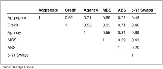
Swap spreads usually are aligned with credit-spreads, although certain factors can cause them to diverge. For example, in a steep yield-curve environment, swapping activity by corporations intensifies, leading to the tightening of swap spreads unaccompanied by the corresponding tightening of credit-spreads. Although such factors weaken the case for swaps as a credit proxy, they promote the role of swaps as a means to diversify systematic risk in total return portfolios. Exhibit 50–4 shows that for the period from July 1992 through October 2010, five-year swaps had a noticeably lower excess return correlation with the Barclays Capital Aggregate Index than did any of the index’s four main spread components. The low excess return correlation implies that adding five-year swaps to a diversified portfolio of agencies, credit, mortgage-backed, and asset-backed securities may reduce risk.

EXHIBIT 50–4
Correlation Matrix: Excess Returns over Treasuries, July 1992–October 2010

The treatment of swaps as a total-return investment should be considered from a tactical as well as a strategic asset allocation perspective. The outperformance and diversification properties that swaps have demonstrated over the recent years make them a valuable tool for total-return portfolio managers.

Credit Default Swaps as Protection against Issuer Risk

Credit default swaps (CDS) have a place in many portfolios. CDS can be used to hedge existing credit exposures in the portfolio and to create new exposures that could not be created otherwise; for example, taking short positions to express a negative view. A conventional cash corporate bond bundles together exposures to interest rates, swap spread, credit-spread (over swaps), and possibly currency risk as well. CDS allow investors to pick from this bundle of exposures only the desired one. With CDS, investors can separate their views on a particular credit (issuer) from views on the market segment to which that issuer belongs.

Besides their primary function of hedging the default risk of particular issuers, CDS are used in a number of other ways. Some investors place bets on the “CDS-cash basis,” that is, the spread between a CDS and corporate debt of the same issuer, or express relative views on two issuers. Finally, CDS are often more liquid than the underlying corporate bonds, providing an easier and cheaper way to get a desired exposure.

QUANTITATIVE METHODS FOR PORTFOLIO OPTIMIZATION

Optimization has been an important part of investment practice since the introduction of mean-variance analysis more than 50 years ago. The asset management problem lends itself quite naturally to optimization techniques. Almost always, it is a multi-variable, multi-constraint task with a well-defined objective. A portfolio of financial assets has two essential characteristics: investment return and risk (i.e., uncertainty about the magnitude of return). Therefore, the countless optimization methods and tools developed over the past decades target one of these two characteristics while controlling the other.

Historically, the usual objective function of portfolio optimization has been to maximize expected return relative to risk. This requires upfront estimates for expected returns of every asset considered in the optimization. As discussed below, historical data, whether long-term or recent, are poor predictors of future performance. Analysts’ forecasts are imperfect as well. This section examines two examples of optimization techniques that do not rely on explicit predictions of asset performance.

Optimal Risk Budgeting Based on Skill

The managing of large, multi-asset portfolios is usually a collective effort. Various managers, analysts, or teams form opinions relevant to particular segments of the overall portfolio. Then all these opinions are considered by some central decision-making authority. This may be a committee of the very same portfolio managers responsible for individual portfolio segments, often supervised by a chief investment officer. Multiple recommendations have to be reconciled: “go long duration,” “overweight the 10-year segment of the curve,” “underweight industrials,” “buy current coupon mortgages,” etc. How can the decision makers establish the magnitudes of exposures along all these dimensions? They need to consider the interaction among all the intended exposures and the resulting overall portfolio risk. But first and foremost, they estimate (explicitly or implicitly) the degree of confidence in each particular recommendation, which depends on the perceived skill of those who made that recommendation.

The manager’s skill is a critical factor that largely determines portfolio performance. While this is obvious, oddly enough, the notion of skill is rarely used formally when allocating portfolio risk or projecting expected outperformance. Even more surprisingly, skill rarely is measured in any disciplined way.

Several studies have examined the role of skill in the historical performance of various investment strategies.²² These skill-based historical simulations produced an interesting conclusion. The information ratios of very diverse strategies were very similar for a given skill level. Apparently, when performance is measured on a risk-adjusted basis, the particular nature of an investment strategy plays a minor role. Performance is essentially determined by the skill and dimensionality (the number of independent decisions) of the strategy.

The empirical results confirm the “Fundamental Law of Active Management” defined by Grinold and Kahn.²³ This law states that the information ratio of an investment strategy is determined by two factors: the “information coefficient” based on correlation between predictions and realizations (and closely related to the probability-based skill) and “breadth” or the number of independent decisions made by the strategy.

Because the information ratio is outperformance (alpha) divided by risk (tracking-error volatility), the law can be expressed slightly differently by stating that a strategy’s alpha is proportional to risk, skill, and the number of independent decisions.

This idea has fundamental implications for portfolio optimization. Asset managers traditionally have used the mean-variance approach to find the optimal asset allocation that maximizes expected outperformance, or alpha, for a given level of risk (or minimizes risk for a given alpha). The Achilles’ heel of this approach is the expected returns of asset classes (or strategies) used in the optimization.

The Barclays Capital proprietary risk-budgeting methodology—ORBS (Optimal Risk Budgeting with Skill)—relies on skill levels, breadth, and directional views to allocate the total risk budget among macro strategies to maximize portfolio alpha. Skill at timing a given strategy is defined as a percentage of directionally correct forecasts for this strategy minus the percentage of directionally wrong forecasts. The risk allocated to an individual strategy is then translated into the size of an active position that corresponds to that risk. At the core of this risk-budgeting methodology is a covariance matrix of returns for the asset classes underlying all considered strategies. This framework is very flexible and can be applied to essentially any set of asset classes and investment strategies with any number of different constraints.

Asset Allocation for Buy-and-Hold Investors

A corporate bond provides investors with a relatively small spread over Treasuries during its lifetime in compensation for the risk of a large, albeit unlikely, loss from default. While default risk is issuer-specific and can be reduced via diversification, correlation of defaults among issuers makes it impossible to eliminate it completely. This asymmetric risk/return profile of credit investing corresponds most closely with the considerations of a long-term investor who intends to hold bonds to maturity. In contrast, most total-return investors have a much shorter time frame and perceive a very different, less asymmetric risk/return profile. For a total-return investor, the dominant risks are spread volatility (essentially symmetric) and possible loss of liquidity. At least in investment-grade markets, credit-quality deterioration typically occurs gradually, so the primary risk for a total-return investor is not default but rather downgrade (and the accompanying spread widening).

This difference in perspective has major implications for buy-and-hold investors. The spreads observed in the market result from interactions among all market participants, many of whom are total-return investors. If these investors expect high short-term spread volatility or liquidity risk, they can drive spreads much wider than would be justified by long-term default risk alone. This action can work to the benefit of long-term credit investors unaffected by short-term risks.

The asymmetric nature of the risk/return profile for long-term investors should be reflected in their asset allocation process. The most common approach to asset allocation, mean-variance optimization, generally is not suitable for buy-and-hold investors. In mean-variance optimization, risk is represented by the standard deviation of asset returns, which implies a symmetric distribution. For very asymmetric return profiles, standard deviation is not a particularly helpful measure of risk. In fact, no single measure of risk is universally appropriate for dealing with extreme, or “tail,” events. The treatment of this “tail risk” must be customized to the needs and risk tolerance of each investor. One approach to asset allocation focuses on the downside risk, that is, the part of the return distribution that is below a certain minimum required return. This approach, though, requires a fuller description of the return distribution; the mean and standard deviation are not sufficient.

The central problem in the buy-and-hold asset allocation process is the fundamental tradeoff between current credit-spreads and expected horizon defaults. When is credit “cheap” from a buy-and-hold perspective? The answer depends on the level of default risk in the portfolio. To what extent can the default risk be reduced by issuer diversification, that is, how many issuers should a portfolio contain to limit default loss to a certain threshold with a given level of confidence? Or what allocation among different credit qualities will maximize spread within a given limit of the tail risk? Sophisticated quantitative models and techniques have been developed to address these matters.²⁴ There is an extensive body of research literature dealing with modeling default risk and particularly with default correlation.

TOOLS FOR QUANTITATIVE PORTFOLIO MANAGEMENT

The challenge for building a good quantitative portfolio-level system comes from the simultaneous need for broad asset class coverage and consistency of analytics across all asset classes. Specialized systems usually offer advanced analytics for specific asset classes. The objective for a portfolio system is to treat a wide range of asset classes within a single consistent framework without giving up too much accuracy.

At the foundation of a powerful analytical suite are basic security-level analytics, such as cash-flow projection, spread-to-price conversion, or duration calculation. The word basic belies the enormous complexity of this task. The variety of financial assets available to investors is ever-expanding and necessitates powerful underlying yield-curve, mortgage-prepayment, option-pricing, and volatility models.

Built on security pricing models is a broad set of portfolio-level analytics, that is, portfolio management tools that help managers analyze portfolio risk exposures, estimate the effect of various changes to portfolio structure, construct optimal portfolios, and attribute achieved performance. An important part of this analytical suite is a multifactor risk model. When such a model is enhanced with optimization capabilities, it becomes a powerful tool for portfolio construction.

A useful complement for history-based risk modeling is flexible scenario analysis. An advanced scenario analysis engine is able to expand a few user-provided inputs into a complete set of maximum-likelihood scenarios for all relevant risk factors. A flexible performance attribution model is another essential component of the analytical suite. Various portfolio optimization tools, such as the risk-budgeting framework described earlier, complete the picture. Each of these building blocks requires sophisticated financial modeling and computer implementation effort. The added challenge is to ensure consistency among all these various tools. The conclusions a manager derives from the risk model should not contradict those from scenario analysis. The ex-post return analysis should attribute the achieved outperformance to the risk exposures highlighted in the ex-ante risk analysis.

KEY POINTS

• Portfolio management entails two essential functions: forming market views at a macro and/or security level and optimally implementing those views in the portfolio.

• Portfolio managers usually focus on the first task. Success in uncovering relative value by market timing, sector, or name selection requires experience and intuition and is usually equated with portfolio management talent.

• Constructing actual portfolios that reflect the desired views is just as vital for ultimate performance. It is this task that is greatly aided by quantitative methods and benefits from the methodologies, tools, and studies described in this chapter.

• Quantitative approaches can add value at each step of the portfolio management process: selection, customization and replication of benchmarks; construction and optimization of benchmarked portfolios; risk analysis; performance attribution; and empirical support of investment decisions.