
CHAPTER
SIXTY-FOUR
THE BASICS OF INTEREST-RATE OPTIONS
Managing Director
Benchmark Solutions
NICHOLAS C. LETICA
Managing Director
Citigroup Global Markets, Inc.
As the sophistication and diversity of investors have grown, the need for derivative instruments such as options has increased accordingly. Knowledge of option strategies, once the province of a few speculators, is now necessary for everyone who wishes to maintain a competitive edge in an increasingly technical market. Moreover, options technology has been applied with increasing success to securities with optionlike characteristics such as callable bonds and mortgage-backed securities.
In Chapter 59, option contracts were described: exchange-traded options on physical securities, exchange-traded options on futures, and over-the-counter (OTC) options. In this chapter we will review how options work, their risk/return profiles, the basic principles of option pricing, and some common trading and portfolio. A more detailed discussion of hedging strategies is provided in Chapter 61.
Throughout most of the discussion, our focus will be on options on physicals. The principles, however, are equally applicable to options on futures or futures options.
HOW OPTIONS WORK
An option is the right but not the obligation to buy or to sell a security at a fixed price. The right to buy is called a call, and the right to sell is called a put; a call makes money if prices rise and a put makes money if prices fall.
If the owner of an option uses the option to buy or to sell the underlying security, we say that the option has been exercised. Because the holder is never required to exercise an option, the holder can never lose more than the purchase price of the option—an option is a limited-liability instrument.
An option on a given security can be specified by giving its strike price and its expiration date. The strike price is the price on the optional purchase. For example, a call with a strike price of par is the right to buy that security at par. The expiration date is the last date on which the option can be exercised: after that, it is worthless, even if it had value on the expiration date. If an option is allowed to expire, it is said to be terminated. On or before the expiration date, the option holder may decide to sell the option for its market value. This is called a pair-off.
Some options can be exercised at any time until expiration: they are called American options. On the other hand, some options can only be exercised at expiration and are called European options. Because it is always possible to delay the exercise of an American option until expiration, an American option is always worth at least as much as its European counterpart. In practice, there are only a limited number of circumstances under which early exercise is advantageous, so the American option rarely costs significantly more than the European.
The easiest way to analyze a position in a security and options on that security is with a profit/loss graph. A profit/loss graph shows the change in a position’s value between the analysis date (“now”) and a horizon date for a range of security prices at the horizon.
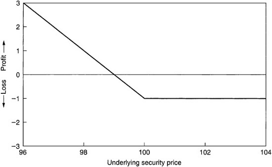
Suppose that a call option struck at par is bought today for 1 point. At expiration, if the security is priced below par, the option will be allowed to expire worthless; the position has lost 1 point. If the security is above par at expiration, the option will be exercised; the position has made 1 point for every point the security is above par, less the initial one-point cost of the option. Exhibit 64–1 shows the resulting profit/loss graph.
EXHIBIT 64–1
Long Call versus Underlying Security Price Call Struck at Par, at Expiration, with 1-Point Premium

Note that if the price of the underlying increases by 1 point, the option purchase breaks even. This happens because the value of the option at expiration is equal to the initial purchase price. A price of 101 is the break-even price for the call: the call purchase will make money if the price of the underlying exceeds 101 at expiration.
A put is the reverse of a call. Look at Exhibit 64–2, which is the profit/loss graph of a put option struck at par bought for 1 point. At expiration, the put is worth nothing if the security’s price is more than the strike price and is worth one point for every point that the security is priced below the strike price. The breakeven price for this trade is 99, so the put purchase makes money if the underlying is priced below 99 at expiration.
EXHIBIT 64–2
Long Put versus Underlying Security Price Put Struck at Par, at Expiration, with 1-Point Premium
Put-Call Parity
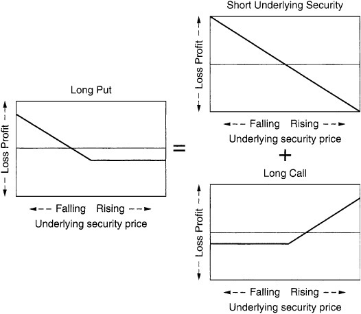
A put and a call struck at-the-money split up the profit/loss diagram of the underlying security into two parts. Consider the position created by buying a call and selling a put such that the strike price of the two options is equal to the price of the underlying. If the price of the security goes up, the call will be exercised; if the price of the security goes down, the put will be exercised. In either case, at expiration the underlying is delivered at the strike price. Thus, in terms of profit and loss, owning the call and selling the put are the same as owning the underlying.
Exhibit 64–3 divides the profit/loss graph of the underlying security into graphs for a long call and a short put, respectively. The following three facts can be deduced:
EXHIBIT 64–3
Long Security = Long Call + Short Put

Long security = long call + short put (Exhibit 64–3)
Long call = long security + long put (Exhibit 64–4)
Long put = short security + long call (Exhibit 64–5)
EXHIBIT 64–4
Long Call = Long Security + Long Put
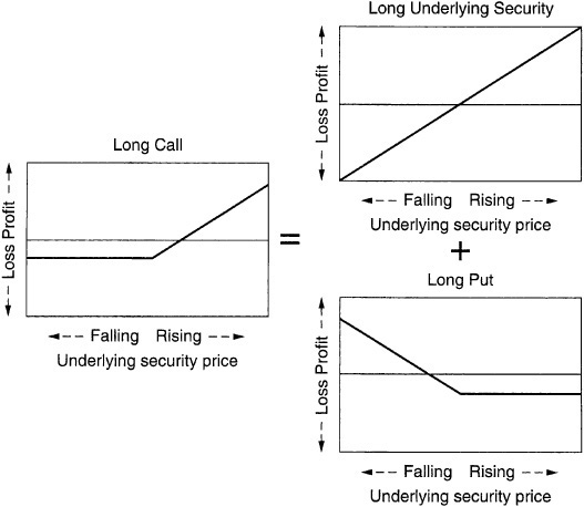
EXHIBIT 64–5
Long Put = Short Security + Long Call
This relationship is called put-call parity; it is one of the foundations of the options markets. Using these facts, a call can be created from a put by buying the underlying, or a put made from a call by selling the underlying. This ability to convert between puts and calls at will is essential to the management of an options position.
Valuing an Option
The first fact to determine about an option is its worth. There are many option valuation models for each class of options, each of which uses different parameters and returns slightly different values. However, the five main determinants of option value are the price of the underlying, the strike price of the option, the expiration of the option, the volatility of the underlying, and the cost of financing the underlying.
The most apparent component of option value is intrinsic value. The intrinsic value of an option is its value if it were exercised immediately. An option with intrinsic value is an in-the-money option. When the underlying security trades right at the strike price, the option is called at-the-money. Otherwise, an option with no intrinsic value is called out-of-the-money.
An option may have value over and above its intrinsic value, called time value. The intrinsic value is the value of the option if exercised immediately, whereas the time value is the remaining value in the option due to time expiration. Clearly, the more time there is to expiration, the greater is the time value.
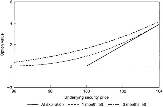
Exhibit 64–6 graphs the value of an option as time to expiration increases. Exhibit 64–7 compares the value of an option at expiration with the values of options with one and three months to expiration. There is a sharp corner in the graph at the strike price that becomes more pronounced as the time to expiration decreases. This sharp corner makes an at-the-money option increasingly difficult to hedge as expiration approaches.
EXHIBIT 64–6
Call Option Value versus Time until Expiration Three Calls: At-the-Money, 1 Point In-the-Money, 1 Point Out-of-the-Money
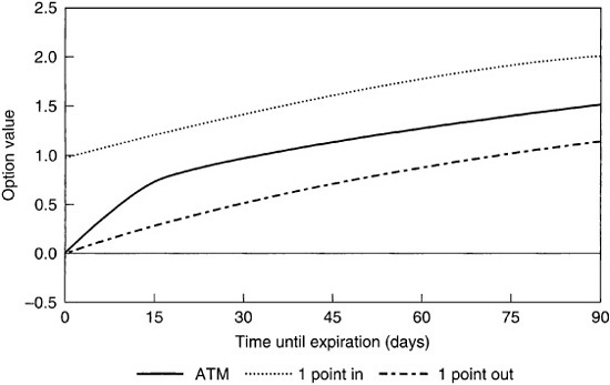
EXHIBIT 64–7
Call Option Value versus Underlying Security Price Call Struck at Par with One and Three Months to Expiration
If the option is out-of-the-money, it has some time value because there is a chance that the option will expire in-the-money; as it gets further out-of-the-money, this is less likely and the time value decreases.
If the option is in-the-money, its time value is due to the fact that it is better to hold the option than the corresponding position in the underlying security because if the security trades out-of-the-money the potential loss on the option is limited to the value of the option; as the option gets further in-the-money, this possibility becomes more farfetched and the time value decreases.
Either way, the time value depends on the probability that the security will trade through the strike price. In turn, this probability depends on how far from the strike price the security is trading and how much the security price is expected to vary until expiration.
Volatility measures the variability of the price or the yield of a security. It measures only the magnitude of the moves, not the direction. Standard option pricing models make no assumptions about the future direction of prices but only about the distribution of these prices. Volatility is the ideal parameter for option pricing because it measures how wide this distribution will be. We discuss volatility in more detail at the end of this chapter.
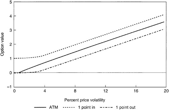
The higher the volatility of a security, the higher is the price of options on that security. If a security had no volatility, for example, that security would always have the same price at time of purchase of an option as at its expiration, so all options would be priced at their intrinsic value. Increasing the volatility of a security increases the time value of options on that security as the chance of the security price moving through the strike price increases. Increases in the value of an at-the-money option are approximately proportional to increases in the volatility of the underlying. Exhibit 64–8 shows how the price of an option behaves as the volatility of the underlying security increases.
EXHIBIT 64–8
Call Option Value versus Percent Price Volatility Three Calls: At-the-Money, 1 Point In-the-Money, 1 Point Out-of-the-Money; Three Months from Expiration
The final factor that influences options prices is the carry on the underlying security. Carry is the difference between the value of the coupon payments on a security and the cost of financing that security’s purchase price. With the usual upward-sloping yield-curve, most securities have a positive carry.
The effect of the carry can be seen by comparing the price of an at-the-money call with an at-the-money put where the underlying security has a positive carry. The writer of the call anticipates the chance of being required to deliver the securities and thus buys the underlying as a hedge; the put writer hedges by selling the underlying. The call writer earns the carry while the put writer loses the carry, so the call should cost less than the put. When the yield-curve inverts and short-term rates are higher than long-term rates, carry becomes negative and calls cost more than puts.
By put-call parity, selling an at-the-money call and buying an at-the-money put are equivalent to shorting the underlying security. The cash taken out of the option trade, accounting for transaction costs, compensates the option holder for the carry on the position in the underlying until expiration. This trade is called a conversion, and it is used frequently to obtain the effect of a purchase or sale of securities when buying or selling the underlying is impossible for accounting reasons.
Exhibit 64–9 compares the cost of an at-the-money call and put for a range of financing rates. The two graphs intersect where the call and the put have the same value: this happens when the cost of financing the underlying is equal to the coupon yield on the security, so the carry is zero and there is no advantage to holding the underlying over shorting it.
EXHIBIT 64–9
Treasury Option Value versus Financing Rate Long Call, Long Put Struck at Par, Three Months to Expiration

Exhibit 64–10 summarizes the parameters that affect the value of an option and how much raising each parameter affects that value.
EXHIBIT 64–10
The Effect of an Increase of a Factor on Option Values

Delta, Gamma, and Theta: Hedging an Option Position
More precise quantitative ways to describe the behavior of an option are needed to manage an option position. Options traders have created the concepts of delta, gamma, and theta for this purpose. Delta measures the price sensitivity of an option, gamma the convexity of the option, and theta the change in the value of the option over time.
For a given option, the delta is the ratio of changes in the value of the option to changes in the value of the underlying for small changes in the underlying. A typical at-the-money call option would have a delta of 0.5; that means for a 1-cent increase in the price of the underlying the value of the call would increase by 0.5 cents. On the other hand, an at-the-money put would have a delta of –0.5; puts have negative deltas because they decrease in value as the price of the underlying increases (see Exhibit 64–10).
The standard method of hedging an options position is called delta hedging, which unsurprisingly makes heavy use of the delta. The idea behind delta hedging is that for small price moves, the price of an option changes in proportion with the change in price of the underlying, so the underlying can be used to hedge the option. For example, 1,000,000 calls with a delta of 0.25 would for small price movements track a position of 250,000 of the underlying bonds, so a position consisting of 1,000,000 of these long calls and 250,000 of the security sold short would be delta-hedged. The total delta of a position shows how much that position is long or short. In the preceding example, the total delta is
0.25 × 1,000,000 – 1 × 250,000 = 0
so the position is neither long nor short.
Intuitively, the delta of an option is the number of bonds that are expected to be delivered into this option. For example, an at-the-money call has a delta of 0.5, which means that one bond is expected to be delivered for every two calls that are held. In other words, an at-the-money call is equally as likely to be exercised as not. An option that is deeply out-of-the-money will have a delta that is close to 0 because there is almost no chance that the option will ever be exercised. An option that is deeply in-the-money almost certainly will be exercised. This means that a deeply in-the-money put has a delta of –1 because it is almost certain that the holder of the option will exercise the put and deliver one bond to the put writer.
Put-call parity tells us that a position in the underlying security may be duplicated by buying a call and selling a put with the same strike price and expiration date. Thus the delta of the call less the delta of the put should be the delta of the underlying. The delta for the underlying is 1, so we get the following equation:
Delta(call) – delta(put) = 1
where call and put are options on the same security with the same strike price and expiration date. This says that once the call is bought and the put sold, the bond is certain to be delivered; if the call is out-of-the-money, the put is in-the-money. Moreover, as the chance of having the underlying delivered into the call becomes smaller, the chance of having to accept delivery as the put is exercised becomes larger. Exhibit 64–11 compares the deltas for a long and a short put.
EXHIBIT 64–11
Option Delta versus Underlying Security Price Long Call, Short Put Struck at Par, Three Months to Expiration

Making the position delta-neutral does not solve all hedging problems, however. This is demonstrated in Exhibit 64–12. Each of the three positions shown is delta-neutral, but position 1 is clearly preferable to position 2, which is, in turn, better than position 3. The difference between these three positions is convexity. A position such as position 1 with a profit/loss graph that curves upward has a positive convexity, whereas position 3 has a graph that curves downward and thus has negative convexity.
EXHIBIT 64–12
Delta-Neutral Positions with Different Gamma

Gamma measures convexity for options; it is the change in the delta for small changes in the price of the underlying. If a position has a positive gamma, then as the market goes up the delta of the position increases and as it declines the delta increases. Such a position becomes longer as the market trades up and shorter as the market trades down. A position like this is called long convexity or long volatility. These names come from the fact that if the market moves in either direction this position will outperform a position with the same delta and a lower gamma. Exhibit 64–13 shows this phenomenon.
EXHIBIT 64–13
Profit/Loss Diagram with Convexity Long Security with Flat and Long Convexity

A long option always has a positive gamma. The delta of a call increases from 0 to 1 as the security trades up, and the delta of a put increases also, moving from –1 to 0. Exhibits 64–1 and 64–2 show that the profit/loss graph of options curves upward. Because of this, options traders often speak of buying or selling volatility as a synonym for buying or selling options.
A position with a zero gamma is called flat convexity or flat gamma. Here, a change in the underlying security price does not change the delta of the position. Such a position trades like a position in the underlying with no options bought or sold. If the position has in addition a delta of zero, then its value is not affected by small changes in the price of the underlying security in either direction. Position 2 in Exhibit 64–12 is a profit/loss graph for a position with no delta or gamma.
A position with negative gamma is called short volatility or short convexity. The profit/loss curve slopes downward in either direction from the current price on the underlying; thus the position gets longer as the market trades down and shorter as the market trades up. Either way, this position loses money if there are significant price movements. Position 3 demonstrates this behavior.
A position that is long volatility is clearly preferable to an otherwise identical position that is short volatility. The holder of the short-volatility position must be compensated for this. In order to create a position that is long volatility it is necessary to purchase options and spend money; moreover, if the market does not move, the values of the options will decrease as their time to expiration decreases, so the position loses money in a flat market.
Conversely, creating a position that is short volatility involves selling options and taking in cash. As time passes, the value of these options sold decreases because their time value falls, so the position makes money in a flat market. Large losses could be sustained in a volatile market, however.
To describe the time behavior of options, there is one last measure called theta. The theta of an option is the overnight change in value of the option if all other parameters (prices, volatilities) stay constant. This means that a long option has a negative theta because as expiration approaches, the time value of the option will erode to zero. For example, a 90-day at-the-money call that costs 2 points might have a theta of –0.45 ticks per day.
Exhibit 64–14 shows the effects of different volatility exposures.
EXHIBIT 64–14
Comparison of Different Volatility Positions (All Positions Are Delta-Neutral)

OPTIONS STRATEGIES—REORGANIZING THE PROFIT/LOSS GRAPH
Investors have many different goals: reducing risk, increasing rates of return, or capturing gains under expected market moves. Often these objectives are simply to rearrange the profit/loss graph of a position in accordance with the investor’s expectations or desires. By increasing the minimum value of this graph, for example, the investor reduces risk.
Options provide a precise tool to accomplish this rearrangement. Because it is impossible to replicate the performance of an option position using just the underlying, options allow a much broader range of strategies to be used. The following characteristics of options provide an explanation.
Directionality
Both a put and a call are directional instruments. A put, for example, performs only in a decreasing market. This property makes options ideal for reducing directional risk on a position. Take, for example, a position that suffers large losses in a downward market and makes a consistent profit if prices rise. By purchasing a put option, some of these profits are given up in exchange for dramatically increased performance if the market declines.
Convexity
Buying and selling options makes it possible to adjust the convexity of a position in almost any fashion. Because OTC options can be purchased for any strike price and expiration, convexity can be bought or sold at any place in the profit/loss graph. For example, an investor holding mortgage-backed securities priced just over par might anticipate that prepayments on this security would start to increase dramatically if the market traded up, attenuating possible price gains. In other words, the investor feels that the position is short convexity above the market. To adjust the profit/loss graph, calls could be purchased with strike prices at or above the market. This trade sells some of the spread over Treasuries in exchange for increased performance in a rising market.
Fee Income
An investor who wishes to increase the performance of a position in a stable market can sell convexity by writing options and taking in fees. This increases the current yield of the position, at the cost of increasing volatility risk in some area of the profit/loss graph. A typical example of this is the venerable covered call strategy, where the manager of a portfolio sells calls on a portion of the portfolio, forgoing some profits in a rising market in exchange for a greater return in a stable or decreasing market.
Leveraged Speculation
Investors with a higher risk/reward profile wish to increase their upside potential and are willing to accept a greater downside risk. In this case, options can be used as a highly leveraged position to capture windfall profits under a very specific market move. A strongly bullish investor might purchase 1-point out-of-the-money calls with 30 days to expiration for ½ point. If the market traded up 2 points by expiration, the option then would be worth 1 point, and the investor would have doubled the initial investment; a corresponding position in the underlying would have appreciated in value by only about 2%. Of course, if the market did not trade up by at least 1 point, the calls would expire worthless.
CLASSIC OPTION STRATEGIES
This section gives a brief explanation of some of the simplest pure options strategies.
Straddle
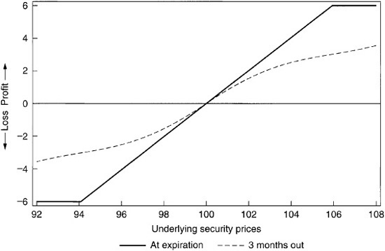
The most pure convexity trade is called a straddle, composed of one call and one put with the same strike price. Exhibit 64–15 shows the profit/loss graph of a straddle struck at-the-money at expiration and with three months to expiration.
EXHIBIT 64–15
Profit/Loss Diagram for a Long Straddle Struck at Par, at Expiration, and Three Months Out
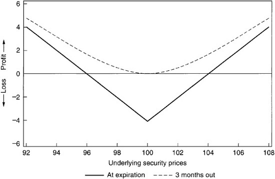
This position is delta-neutral because it implies no market bias. If the market stays flat, the position loses money as the options’ time value disappears by expiration. If the market moves in either direction, however, either the put or the call will end up in-the-money, and the position will make money. This strategy is most useful for buying convexity at a specific strike price. Investors who are bearish on volatility and anticipate a flat market could sell straddles and make money from time value.
Strangle
A strangle is the more heavily leveraged cousin of a straddle. An at-the-money strangle is composed of an out-of-the-money call and an out-of-the-money put. The options are struck so that they are both equally out-of-the-money, and the current price of the security is halfway between the two strikes. The profit/loss graph is found in Exhibit 64–16.
EXHIBIT 64–16
Profit/Loss Diagram for a Long Strangle Struck at Par, at Expiration, and Three Months Out
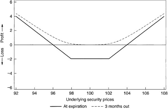
Just like a straddle, a strangle is a pure volatility trade. If the market stays flat, the position loses time value, whereas if the market moves dramatically in either direction the position makes money from either the call or the put. Because the options in this position are both out-of-the-money, the market has to move significantly before either option moves into the money. The options are much cheaper, however, so it is possible to buy many more options for the same money. This is the ideal position for the investor who is heavily bullish on volatility and wants windfall profits in a rapidly moving market.
Writing strangles is a very risky business. Most of the time the market will not move enough to put either option much into the money, and the writer of the strangle will make the fee income. Occasionally, however, the market will plummet or spike, and the writer of the strangle will suffer catastrophic losses. This accounts for the picturesque name of this trade.
Spread Trades
Spread trades involve buying one option and funding all or part of this purchase by selling another. A bull spread can be created by owning the underlying security, buying a put struck below the current price, and selling a call above the current price. Because both options are out-of-the-money, it is possible to arrange the strikes so that the cost of the put is equal to the fee for the call. If the security price falls below the put strike or rises above the call strike, the appropriate option will be exercised and the security will be sold. Otherwise, any profit or loss will just be that of the underlying security. In other words, this position is analogous to owning the underlying security except that the final value of the position at expiration is forced to be between the two strikes. Exhibit 64–17 shows the profit/loss graph of this position at expiration and with three months left of time value.
EXHIBIT 64–17
Profit/Loss Diagram for a Bull Spread Struck at Par, at Expiration, and Three Months Out
The other spread trade is a bear spread: It is the reverse of a bull spread. It can be created by selling a bull spread. Using put-call parity, it also can be set up by holding the underlying security, buying an in-the-money put, and selling an in-the-money call. A bear spread is equivalent to a short position in the underlying, where the position must be closed out at a price between the two strike prices. Exhibit 64–18 shows the profit/loss graph of a bear spread.
EXHIBIT 64–18
Profit/Loss Diagram for a Bear Spread Struck at Par, at Expiration, and Three Months Out

PRACTICAL PORTFOLIO STRATEGIES
The strategies discussed in the preceding section are the basic techniques used by speculators to trade options. The usual fixed income investor has a lower risk/reward profile than the speculator and specific objectives that must be accomplished; a floor on rate of return or an increase in current yield, for example. Such investors need a class of strategies different from that needed by speculators; even though the same strategies are often used, the risk is carefully controlled.
Portfolio Insurance
This is the most obvious and one of the most commonly used options strategies. An investor with a portfolio of securities who fears a decreasing market buys puts on some or all of the portfolio; if the market falls, the puts are exercised, and the securities are sold at the strike price. Alternatively, the investor may keep the underlying security and pair off the in-the-money puts, receiving cash in compensation for the decreased value of the security. Either way, the investor has limited losses on the portfolio in exchange for selling off return in a stable or rising market.
As the strike price of the put increases, so does its cost and the resulting impact on the stable market rate of return. Often, out-of-the-money options are used; the floor on returns is lower because the strike price is lower, but the lower cost of the options means that less return is given up if the market is flat or rises. By put-call parity, such a position is equivalent to holding a call option struck at or in-the-money.
Another popular strategy is to buy at-the-money options on a portion of the portfolio. This reduces but does not eliminate downside risk: Exhibit 64–19 shows the profit/loss graphs at expiration for positions with different percentages of the portfolio hedged with an at-the-money put. Note that all the graphs intersect at a single point. This is the point where the initial cost of the option is equal to the value of the option at expiration, which is the break-even price for this trade.
EXHIBIT 64–19
Hedged Underlying Security with Puts Long Puts Struck at Par, at Expiration

It is not possible to buy options on many classes of securities that may well be held in a portfolio. Perfect insurance for such securities is unattainable, but cross-market hedging often will permit a reduction in downside risk to acceptable levels.
Covered Calls
Writing covered calls is a strategy that sells volatility in return for fees. An investor who holds a portfolio sells calls on some or all of the portfolio in return for fees. If the market stays the same or falls, the investor pockets the option fees. If the market increases until the calls are in-the-money, the investor is called out by the option holder. In other words, possible gains on the portfolio are sold for fee income.
Often the investor wishes to preserve some upside potential. Just as in the portfolio insurance example, there are two different ways to do this. The calls can be struck out-of-the-money, that is, above the current market price. This strategy allows all gains up to the strike price to be captured. If the bonds in the portfolio are currently trading below the original purchase price, a popular strategy is to sell calls struck at this purchase price. This provides fee income and increased current yield but prevents the possibility that the bonds will be called at a price below the original purchase price and the portfolio will book a capital loss.
Otherwise, calls can be sold on a portion of the portfolio. This allows unlimited price gains to be captured on the remainder. Exhibit 64–20 shows the profit/loss graph of a covered call program where different portions of the portfolio have calls sold against them.
EXHIBIT 64–20
Covered Call Writing Program Short Calls Struck at Par, at Expiration

Buy-Writes and Writing Puts
Buy-writes and writing puts are two very closely related strategies for selling volatility that most investors think of as entirely different. To execute a buy-write, a bond is purchased, and simultaneously, a call is written on this bond to the same dealer for the fee income. If the security is trading above the strike price at expiration, the security is called, and the investor is left with just the option fee. If the price of the security has fallen, the investor is left holding the security, but the total cost of the security is reduced by the fee from the call. By put-call parity, this trade is identical to writing a put struck at-the-money. In both cases, the investor is delivered the security only if the price of the security is lower than the price of the original sale.
In the MBS market, a buy-write is composed of forward purchases and short calls on forward delivery contracts (standard TBA transactions). If the call is exercised, it offsets the forward sale, and the buyer never takes delivery of the security, keeping the fee income. Otherwise, the buyer will receive the security on the forward settlement date for the original forward sale price, although the total price is decreased by the value of the option fee.
Put writing is a more general strategy that applies to all fixed income options markets. The investor writes a put for the fee income and receives the underlying instrument at expiration if the security trades below the strike price. This can be a very effective strategy if carefully structured. An investor may feel that a security offers real value if bought at a certain price below the market. The investor could then write puts struck at that price. If the security falls below the strike, it is delivered at a price that is more agreeable than the current price. Otherwise, the investor simply pockets the fee income.
VOLATILITY
Volatility plays a key role in the valuation of options and in option strategies. In this section we focus on methods for estimating volatility.
Statistically, volatility is a measure of the dispersion or spread of observations around the mean of the set of observations. If volatility seems strangely like a standard deviation, then you remember your statistics. When people speak of volatility, all they really are talking about is a standard deviation.
For fixed income securities, volatility is expressed in yield or price units, either on a percentage or on an absolute basis. Price volatilities can be computed for any security. Yield volatilities should be computed only for those securities with a consistent method for computing yield. Given the complexity of calculating a yield on a MBS and the variation of results, the predominant volatility measure in the MBS market is price volatility. The government bond market, where yields are easily calculated, favors yield volatility.
There are two types of volatility: empirical volatility and implied volatility. Each is described below.
Empirical Volatility
Empirical volatility is the actual, historical market volatility of a specific security. These numbers typically are calculated for various time periods (10 days, 30 days, 360 days) and usually are annualized.1 Calculating an empirical volatility is nothing more than calculating the standard deviation of a time series. Thus an absolute volatility is the annualized standard deviation of daily price or yield changes, assuming a normal distribution.
Percentage volatility is the annualized standard deviation of the daily change in the log of prices or yields, assuming a lognormal distribution of prices or yields. Similar to the daily absolute yield changes, the logs of the daily yield changes have a slight bias toward lower yields. The intuitive approach to calculating a percentage volatility is to find the standard deviation of daily returns, assuming a normal distribution. This approach is equivalent to the lognormal assumption as long as the distribution can be characterized as being equally normal and log normal and, the changes in prices are taken on a small interval, such as daily.
As mentioned previously, empirical volatility can be measured over various time periods. The most common interval on which the standard deviation is taken is 30 days; other common intervals are 10 days and 360 days. The choice of interval determines how quickly and to what degree an empirical volatility responds to deviations. As the time period shortens, volatility increasingly reflects current conditions but is more unstable as each sample asserts greater influence in the deviation. Conversely, as the interval increases, more of a lag and a smoothing are introduced into the calculation.
The interval used to calculate an empirical volatility should be chosen to match the length of the option contract. This provides the investor with an indication of how volatile the underlying security has been recently and how this relates to the volatility employed to price the option.
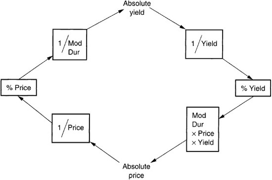
With no industry standard for volatility units, converting between the price and yield expression of absolute or percentage volatility is a useful skill. The path to follow to convert from one unit to the next is shown in Exhibit 64–21. The modified duration of a security provides the link between price and yield volatilities. Modified duration is defined as the percentage change in price divided by the absolute change in yield.
Implied Volatility
Implied volatility is merely the market’s expectation of future volatility over a specified time period. An option’s price is a function of the volatility employed, so where an option’s price is known, the implied volatility can be derived. Although it sounds straightforward, calculating an implied volatility is far more complicated than calculating an empirical volatility because expectations cannot be observed directly. An option pricing model along with a mathematical method to infer the volatility must be employed. The result of this calculation is a percentage price volatility that can be converted to the various types of volatility measures discussed previously (see Exhibit 64–21).
EXHIBIT 64–21
Converting Volatility Measures
Owing to the existence and liquidity of fixed income options, proxies for implied volatilities can be derived from Treasuries. Options on Treasury futures listed on the Chicago Board of Trade (CBOT) are often the best vehicles for implied volatility calculations. The resulting implied volatility provides a good indication of the market’s expected volatility for the Treasuries with maturities similar to that of the particular bond futures contract in question. The implied volatility on the 10-year bond futures contract, for example, is a useful proxy for the market’s expected volatility on intermediate-term Treasury securities.
KEY POINTS
• An option is the right but not the obligation to buy (a call option) or to sell (a put option) a security at a fixed price (strike price or exercise). The expiration date is the last date on which the option can be exercised. Some options can be exercised at any time until expiration (American options); some options can only be exercised at expiration (European options).
• The relationship among the price of a security, the price of a put, and the price of a call is called the put-call parity and is one of the foundations of the options markets.
• The price of an option is the sum of its intrinsic value and time value.
• Volatility measures the variability of the price or the yield of a security. It measures only the magnitude of the moves, not the direction. Standard option pricing models make no assumptions about the future direction of prices but only about the distribution of these prices. Volatility is the parameter used for option pricing because it measures how wide this distribution will be. The higher the volatility of a security, the higher is the price of options on that security.
• To manage an option position, quantitative ways to describe the behavior of an option are needed. These include an options delta, gamma, and theta.
• Any investor with specific goals can use option strategies to tailor the performance of a portfolio.
• Because it is impossible to obtain the effects of options by using only the underlying securities, a whole new universe of strategic possibilities is opened up. In particular, investors with contingent liabilities cannot create an adequate hedge without the use of options.
• Increased liquidity in the options markets and a better understanding of the properties of options make option strategies more accessible to the average investor and allow these strategies to be used for a wider range of securities. In particular, the over-the-counter options markets allow the purchase and sale of options with any desired strike price and expiration date.
• Refinements to option valuation technology continue to improve cross-market arbitrage trades where securities and options in one market can duplicate securities in another. As options trading removes the arbitrages, the relationships among the various markets are reinforced.