
14. Subqueries
In Chapter 4, we talked about composite functions as functions that contain other functions. In a similar manner, A SQL query can contain other queries. Queries contained within other queries are called subqueries.
The topic of subqueries is somewhat complex, primarily because there are many different ways in which they can be used. Subqueries can be found in many different parts of the SELECT statement, each with different nuances and requirements. Additionally, as a query contained within another query, a subquery can be related to and dependent on the main query, or it can be completely independent of the main query. Again, this distinction results in different requirements for their usage.
No matter how subqueries are used, they add a great deal of flexibility to the ways in which you can write SQL queries. Often, subqueries provide functionality that could be accomplished by other means. In such instances, personal preference will come into play as you decide whether or not to utilize the subquery solution. However, as you’ll see, there are certain situations for which subqueries are absolutely essential for the task at hand.
With that said, let’s begin our discussion with an outline of the basic types of subqueries.
Types of Subqueries
Subqueries can be used not only with SELECT statements but also with the INSERT, UPDATE, and DELETE statements that will be covered in Chapter 17, “Modifying Data.” In this chapter, however, we’ll restrict our discussion of subqueries to the SELECT statement.
Here’s the general SELECT statement we’ve seen previously:
SELECT columnlist
FROM tablelist
WHERE condition
GROUP BY columnlist
HAVING condition
ORDER BY columnlist
Subqueries can be inserted into virtually any of the clauses in the SELECT statement. However, the way in which the subquery is stated and used varies slightly, depending on whether it is used in a columnlist, tablelist, or condition.
But what exactly is a subquery? A subquery is merely a SELECT statement that has been inserted inside another SQL statement. The results returned from the subquery are used within the context of the overall SQL query. Additionally, there can be more than one subquery in a SQL statement. To summarize, subqueries can be specified in three different ways:
![]() When a subquery is part of a tablelist, it specifies a data source. This applies to situations where the subquery is part of a FROM clause.
When a subquery is part of a tablelist, it specifies a data source. This applies to situations where the subquery is part of a FROM clause.
![]() When a subquery is part of a condition, it becomes part of the selection criteria. This applies to situations where the subquery is part of a WHERE or HAVING clause.
When a subquery is part of a condition, it becomes part of the selection criteria. This applies to situations where the subquery is part of a WHERE or HAVING clause.
![]() When a subquery is part of a columnlist, it creates a single calculated column. This applies to situations where the subquery is part of a SELECT, GROUP BY, or ORDER BY clause.
When a subquery is part of a columnlist, it creates a single calculated column. This applies to situations where the subquery is part of a SELECT, GROUP BY, or ORDER BY clause.
The remainder of this chapter explains each of these three scenarios in detail.
Subqueries as a Data Source
When a subquery is specified as part of the FROM clause, it instantly creates a new data source. This is similar to the concept of creating a view and then referencing that view in a SELECT. The only difference is that a view is permanently saved in a database. A subquery used as a data source isn’t saved. It exists only temporarily, as part of the SELECT statement. Nevertheless, you can think of a subquery in a FROM clause as a type of virtual view.
Let’s first consider an example that illustrates how subqueries can be used as a data source. To illustrate the use of subqueries in this chapter, we will reference this Users table:
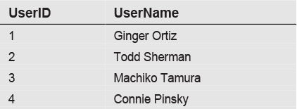
We will also reference this Transactions table, related to the Users table by UserID:
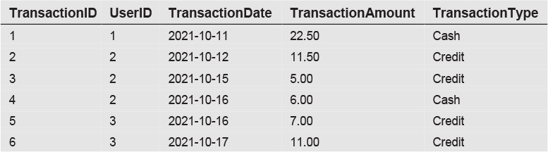
This data is actually quite similar to the Customers and Orders tables we’ve seen in previous chapters. The Users table resembles the Customers table, except that we’ve combined the first and last names into a single column. The Transactions table has entries similar to orders, except that we’ve added a TransactionType column to indicate whether the transaction is cash or credit.
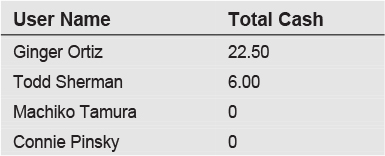
To begin, we would like to see a list of users, along with a total sum of the cash transactions they have placed. The following SELECT accomplishes that task:
SELECT
UserName AS ‘User Name’,
ISNULL(CashTransactions.TotalCash, 0) AS ‘Total Cash’
FROM Users
LEFT JOIN

(SELECT
UserID,
SUM(TransactionAmount) AS ‘TotalCash’
FROM Transactions
WHERE TransactionType = ‘Cash’
GROUP BY UserID) AS CashTransactions

ON Users.UserID = CashTransactions.UserID
ORDER BY Users.UserID
Two blank lines were inserted to clearly separate the subquery from the rest of the statement. The subquery is the middle section of the statement. The results are:
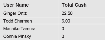
Connie Pinsky shows no cash transactions, because she made no transactions at all. Although Machiko Tamura has two transactions, they were both credit transactions, so she also shows no cash. Note that the ISNULL function converts the NULL values that would normally appear for Machiko and Connie to a 0.
Let’s now analyze how the subquery works. The subquery in the previous statement is:
SELECT
UserID,
SUM(TransactionAmount) AS ‘TotalCash’
FROM Transactions
WHERE TransactionType = ‘Cash’
GROUP BY UserID
In general form, the main SELECT statement in the above is:
SELECT
UserName AS ‘User Name’
ISNULL(CashTransactions.TotalCash, 0) AS ‘Total Cash’
FROM Users
LEFT JOIN (subquery) AS CashTransactions
ON Users.UserID = CashTransactions.UserID
ORDER BY Users.UserID
If the subquery were executed on its own, the results would be:
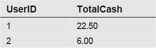
We see data for only users 1 and 2. The WHERE clause in the subquery enforces the requirement that we look only at cash orders.
The entire subquery is then referenced as if it were a separate table or view. Notice that the subquery is given a table alias of CashTransactions. This allows the columns in the subquery to be referenced in the main SELECT. As such, the following line in the main SELECT references data in the subquery:
ISNULL(CashTransactions.TotalCash, 0) AS ‘Total Cash’
CashTransactions.TotalCash is a column taken from the subquery.
You might ask whether it was truly necessary to use a subquery to obtain the desired data. In this case, the answer is that it was. We might have attempted to simply join the Users and Transactions tables via a LEFT JOIN, as in the following:
SELECT
UserName AS ‘User Name’,
SUM(TransactionAmount) AS ‘Total Cash Transactions’
FROM Users
LEFT JOIN Transactions
ON Users.UserID = Transactions.UserID
WHERE TransactionType = ‘Cash’
GROUP BY Users.UserID, Users.UserName
ORDER BY Users.UserID
However, this statement yields the following data:

We no longer see any rows for Machiko Tamura or Connie Pinsky, because the WHERE clause exclusion for cash orders is now in the main query rather than in a subquery. As a result, we don’t see any data for people who didn’t place cash orders.
Subqueries as Selection Criteria
In Chapter 7, “Boolean Logic,” we introduced the first format of the IN operator. The example we used was:
WHERE State IN (‘IL’, ‘NY’)
In this format, the IN operator merely lists a number of values in parentheses. We now want to introduce a second format for the IN, in which an entire SELECT statement is inserted inside the parentheses. For example, a list of states might be specified as:
WHERE State IN
(SELECT
States
FROM StateTable
WHERE Region = ‘Midwest’)
Rather than list individual states, this second format allows us to generate a dynamic list of states through more complex logic.
Let’s illustrate with an example that uses the Users and Transactions tables. In this scenario, we want to retrieve a list of users who have ever paid cash for any transaction. A SELECT that accomplishes this is:
SELECT UserName AS ‘User Name’
FROM Users
WHERE UserID IN
(SELECT UserID
FROM Transactions
WHERE TransactionType = ‘Cash’)
The resulting data is:

Machiko Tamura is not included in the list because, although she has transactions, none of them were in cash. Notice that the subquery SELECT is placed entirely within the parentheses for the IN keyword. There is only one column, UserID, in the columnlist of the subquery. This is a requirement, because we want the subquery to produce the equivalent of a list of values for only one column. Also note that the UserID column is used to connect the two queries. Although we’re displaying UserName, we’re using UserID to define the relationship between the Users and Transactions tables.
Once again, we can ask whether it was necessary to use a subquery, and this time the answer is that it was not. Here is an equivalent query that returns the same data.
SELECT UserName AS ‘User Name’
FROM Users
INNER JOIN Transactions
ON Users.UserID = Transactions.UserID
WHERE TransactionType = ‘Cash’
GROUP BY Users.UserName
Without using a subquery, we can directly join the Users and Transactions tables. However, a GROUP BY clause is now needed to ensure that we bring back only one row for each user.
Correlated Subqueries
The subqueries we’ve seen so far have been uncorrelated subqueries. Generally speaking, all subqueries can be classified as either uncorrelated or correlated. These terms describe whether the subquery is related to the query in which it is contained. Uncorrelated subqueries are unrelated. When a subquery is unrelated, that means it is completely independent of the outer query. Uncorrelated subqueries are evaluated only once as part of the entire SELECT statement. Furthermore, uncorrelated subqueries can stand on their own. If you wanted to, you could execute an uncorrelated subquery as a separate query.
In contrast, correlated subqueries are specifically related to the outer query. Because of this explicit relationship, correlated subqueries must be evaluated for each row returned and can produce different results each time the subquery is invoked. Correlated subqueries can’t be executed on their own, because some element in the query makes it dependent on the outer query.
The best way to explain is with an example. Returning to the Users and Transactions tables, let’s say we want to produce a list of users who have a total transaction amount less than twenty dollars. Here’s a statement that accomplishes that request:
SELECT
UserName AS ‘User Name’
FROM Users
WHERE
(SELECT
SUM(TransactionAmount)
FROM Transactions
WHERE Users.UserID = Transactions.UserID)
< 20
The result is:

What makes this subquery correlated, as opposed to uncorrelated? The answer can be seen by looking at the subquery itself:
SELECT
SUM(TransactionAmount)
FROM Transactions
WHERE Users.UserID = Transactions.UserID
This subquery is correlated because it cannot be executed on its own. If run by itself, this subquery would produce an error because the Users.UserID column in the WHERE clause doesn’t exist within the context of the subquery. To understand what’s going on, it’s helpful to look at the entire SELECT statement in a more general way:
SELECT
UserName AS ‘User Name’
FROM Users
WHERE
SubqueryResult < 20
The subquery returns a columnlist with a single value, which we’re calling SubqueryResult. As a correlated subquery, the subquery must be evaluated for each user. Also, note that this type of subquery demands that it only returns a single row and a single value. The SubqueryResult could not be evaluated if there were more than one row or value involved.
As before, you might ask whether a subquery was necessary, and once again the answer is that it was not. Here’s an equivalent statement that produces the same result:
SELECT
UserName AS ‘User Name’
FROM Users
LEFT JOIN Transactions
ON Users.UserID = Transactions.UserID
GROUP BY Users.UserID, Users.UserName
HAVING SUM(TransactionAmount) < 20
Notice, however, that without a subquery, the equivalent statement now requires GROUP BY and HAVING clauses. The GROUP BY clause creates groups of users, and the HAVING clause enforces the requirement that each group must have transacted less than twenty dollars.
Focus on Analysis: Moving Averages
Correlated subqueries can be used to compute a moving average for a set of data. We’ll illustrate this capability using the Transactions table seen in this chapter. In this scenario, we want to compute the average Transaction Amount for each row and all other rows that are either on that same day, one day before, or one day after. This is a SELECT that accomplish that task:
SELECT
A.TransactionDate,
A.TransactionAmount,
(SELECT
SUM (B.TransactionAmount) / COUNT(B.TransactionAmount)
FROM Transactions AS B
WHERE DATEDIFF(day, A.TransactionDate, B.TransactionDate)
BETWEEN -1 AND 1)
AS ‘Moving Average’
FROM TRANSACTIONS AS A
ORDER BY A.TransactionDate
The output of this statement is:
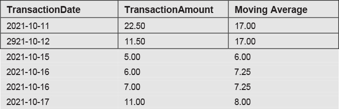
To understand how this query works, let’s focus on the subquery:
(SELECT
SUM (B.TransactionAmount) / COUNT(B.TransactionAmount)
FROM Transactions AS B
WHERE DATEDIFF(day, A.TransactionDate, B.TransactionDate)
BETWEEN -1 AND 1)
This is a correlated subquery because it refers to data in the outer query and cannot be run on its own. Note that table aliases are used to distinguish between the Transactions table in the outer query (named A) from the Transactions table in the subquery (named B). In the subquery, we use the DATEDIFF function to calculate the number of days between the A.TransactionDate and B.TransactionDate. The BETWEEN operator ensures that we only select subquery rows that are within 1 day prior and 1 day after the TransactionDate. The average for those rows is computed as the SUM of all such rows divided by the the COUNT of those rows. This is the moving average.
The EXISTS Operator
An additional technique associated with correlated subqueries utilizes a special operator called EXISTS. This operator allows you to determine whether data in a correlated subquery exists. To illustrate, let’s say that we want to discover which users have made any transactions. This can be accomplished with the use of the EXISTS operator in this statement:
SELECT
UserName AS ‘User Name’
FROM Users
WHERE EXISTS
(SELECT *
FROM Transactions
WHERE Users.UserID = Transactions.UserID)
This statement returns:

This is a correlated subquery because it cannot be executed on its own without reference to the main query. The EXISTS keyword in the above statement is evaluated as true if the SELECT in the correlated subquery returns any data. Notice that the subquery selects all columns (SELECT *). Because it doesn’t matter which particular columns are selected in the subquery, we use the asterisk to return all columns. We’re interested only in determining whether any data exists in the subquery. The result is that the query returns all users except Connie Pinsky. She doesn’t appear because she has no transactions.
As before, the logic in this statement can be expressed in other ways. Here’s a statement that obtains the same results by using a subquery with the IN operator:
SELECT
UserName AS ‘User Name’
FROM Users
WHERE UserID IN
(SELECT UserID
FROM Transactions)
This statement is probably easier to comprehend.
Here’s yet another statement that retrieves the same data without the use of a subquery:
SELECT
UserName AS ‘User Name’
FROM Users
INNER JOIN Transactions
ON Users.UserID = Transactions.UserID
GROUP BY UserName
In this statement, the INNER JOIN enforces the requirement that the user must also exist in the Transactions table. Also note that this query requires the use of a GROUP BY clause to avoid returning more than one row per user.
Subqueries as a Calculated Column
The final general use of subqueries is as a calculated column. Suppose we would like to see a list of users, along with a count of the number of transactions they have placed. This can be accomplished without subqueries using this statement:
SELECT
UserName AS ‘User Name’,
COUNT(TransactionID) AS ‘Number of Transactions’
FROM Users
LEFT JOIN Transactions
ON Users.UserID = Transactions.UserID
GROUP BY Users.UserID, Users.UserName
ORDER BY Users.UserID
The output is:
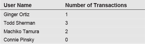
Notice that we used a LEFT JOIN to accommodate users who may not have made any transactions. The GROUP BY enforces the requirement that we end up with one row per user. The COUNT function produces a count of the number of rows in the Transactions table.
Another way of obtaining the same result is to use a subquery as a calculated column. This looks like the following:
SELECT
UserName AS ‘User Name’,
(SELECT
COUNT(TransactionID)
FROM Transactions
WHERE Users.UserID = Transactions.UserID)
AS ‘Number of Transactions’
FROM Users
ORDER BY Users.UserID
In this example, the subquery is a correlated subquery. The subquery cannot be executed on its own, because it references a column from the Users table in the WHERE clause. This subquery returns a calculated column for the SELECT columnlist. In other words, after the subquery is evaluated, it returns a single value, which is then included in the columnlist. Here’s the general format of the previous statement:
SELECT
UserName AS ‘User Name’,
SubqueryResult AS ‘Number of Transactions’
FROM Users
ORDER BY Users.UserID
As seen, the entire subquery returns a single value, which is used for the Number of Transactions column.
Common Table Expressions
An alternate subquery syntax allows it to be defined explicitly prior to the execution of the main query. This is known as a common table expression. In this syntax, the entire subquery is removed from its normal location and stated at the top of the query. The WITH keyword is used to indicate the presence of a common table expression. Although they may be used with correlated subqueries, a common table expression is far more useful for uncorrelated subqueries. To illustrate, let’s return to the first subquery presented in this chapter:
SELECT
UserName AS ‘User Name’,
ISNULL(CashTransactions.TotalCash, 0) AS ‘Total Cash’
FROM Users
LEFT JOIN

(SELECT
UserID,
SUM(TransactionAmount) AS ‘TotalCash’
FROM Transactions
WHERE TransactionType = ‘Cash’
GROUP BY UserID) AS CashTransactions

ON Users.UserID = CashTransactions.UserID
ORDER BY Users.UserID
As seen, the subquery in the above statement is given an alias of CashTransactions, and is joined to the Users table on the UserID column. The purpose of the subquery is to provide a total of the cash transactions for each user. The output of this query is:
We’ll now present an alternate way of expressing this same logic, using a common table expression. The query looks like this:
WITH CashTransactions AS
(SELECT
UserID,
SUM(TransactionAmount) as TotalCash
FROM Transactions
WHERE TransactionType = ‘Cash’
GROUP BY UserID)

SELECT
UserName AS ‘User Name’,
ISNULL(CashTransactions.TotalCash, 0) AS ‘Total Cash’
FROM Users
LEFT JOIN CashTransactions
ON Users.UserID = CashTransactions.UserID
ORDER BY Users.UserID
In this alternative expression, the entire subquery has been moved to the top, prior to the main SELECT query. The WITH keyword tells us that a common table expression follows. The first line indicates that CashTransactions is an alias for the common table expression. The common table expression follows the AS keyword and is enclosed within parentheses.
We’ve inserted a blank line to separate the common table expression from the primary query. The following line in the main query:
LEFT JOIN CashTransactions
initiates the outer join to the common table expression, which is referenced via the CashTransactions alias. The chief virtue of the common table expression is its simplicity. The main query becomes easier to comprehend, because the details of the subquery now appear as a separate entity. The output of this query with a common table expression is identical to the original query with a subquery.
It’s really a matter of personal preference as to whether you’d like to use common table expressions in your queries. Whereas subqueries are embedded in a larger query, common table expressions state the subqueries up front.
Looking Ahead
In this chapter, we’ve seen subqueries used in three different ways: as a data source, in selection criteria, and as a calculated column. Additionally, we’ve seen examples of both correlated and uncorrelated subqueries. Finally, we briefly demonstrated the use of an alternate method of expressing subqueries using the common table expression. As such, we’ve really only touched on some of the uses of subqueries. What complicates the matter is that many subqueries can be expressed in other ways. Whether or not you choose to use subqueries depends on your personal taste and sometimes on the performance of the statement.
Through our use of joins and subqueries, we’ve explored numerous ways to select data from multiple tables. In our next chapter, “Set Logic,” we’ll look at a method of combining entire queries into a single SQL statement. This is a special type of logic that allows us to merge multiple data sets into a single result. As you’ll see, set logic procedures are sometimes necessary in order to display sets of data that are only partially related to each other. As with subqueries, the techniques of set logic provide additional flexibility and logical possibilities for your SQL statements.
Subqueries as Selection Criteria
Subqueries as a Calculated Column