
System performance measurements
U. Herrmann*; D. Kearney†; M. Röger‡; C. Prahl‡ * Solar-Institute Jülich, FH Aachen—University of Applied Sciences, Jülich, Germany
† Kearney & Associates, Vashon, WA, United States
‡ German Aerospace Center (DLR), Almería, Spain
Keywords
Performance measurement; Acceptance tests; Plant efficiency; Test code and standards
Prior to commercial operation, large solar systems in utility-size power plants need to pass performance acceptance tests conducted by the engineering, procurement, and construction (EPC) contractor or owners. Test procedures for this purpose must yield results of a high level of accuracy consistent with good engineering knowledge and practice, guided by international test standards when available. Parabolic trough and solar tower systems are typical of such solar systems. The power block and balance of plant, which may be included in the performance test, are conventional technology. Performance tests are also useful during technology development, optimization, and monitoring.
This chapter introduces performance and acceptance testing procedures, and describes state-of-the-art tools, methods, and instruments to accomplish those objectives.
5.1 Introduction
5.1.1 Unique characteristics of solar power plant performance
The difference between a solar power plant and a conventional fossil-fired plant is the source of the heat supply to drive the turbine cycle. In fossil-fired plants, the heat is supplied by burning a fossil fuel such as coal, oil, or gas. The (fossil) heat input can be controlled very well and the turbine cycle can be operated in stable and controllable conditions.
This is fundamentally different for solar thermal power plants. The heat supply for solar power plants comes not from a chemical reaction (the combustion process of fuels), but from a conversion of electromagnetic waves emitted by the sun into heat. In order to reach the required temperatures to drive a turbine cycle, the solar radiation has to be concentrated. An optical device is required to capture the sun and concentrate the solar radiation onto a focal area where the electromagnetic radiation is absorbed and converted into heat. In order to reach high conversion efficiency, a good understanding of the optical characteristics of those concentrators is essential. The concentrator or solar collector is composed of different components that are described in Part 1 of this book. Tests of individual components can generally be performed in workshops or laboratories, whereas the tests described in this part refer to larger subsystems and complete systems that can only be assembled and tested on site. Optical systems tests of the concentrators are described in Section 5.2 of this chapter.
In addition to the different nature of the energy conversion process, the second and even more critical difference is the fluctuating nature of the energy input by the sun. Unlike the fossil fuel input into fossil-fired plants, the energy source of a solar power plant cannot be controlled. The continuous movement of the sun relative to the earth leads to a continuous change of heat input to the solar field even at good weather conditions, as shown in Fig. 5.1.

In addition to this regular continuous change caused by the relative movement of the sun, additional fluctuation can be caused by cloudy weather conditions. Thus, the solar field has to deal with transient, fluctuating, and noncontrollable heat inputs. The consequences of these effects are intensified by the large dimensions of a solar field. For example, solar thermal trough power plants are being constructed with large turbine capacities up to 280 MWe gross and, if significant thermal storage is included in the system, can require solar fields up to about 2.6 million m2 of reflector aperture even in areas of high solar resource. Consequently, the solar input can even vary along the field when clouds are passing. As a result, the thermal and electrical output of the plant cannot always be kept constant, and might fluctuate.
Therefore, standard performance tests for the assessment of the thermal and electrical performance developed for fossil-fired plants and also used for acceptance testing that are based on steady-state conditions cannot be applied to solar power plants. While measurement devices used for testing are mostly standard instruments, specific test and evaluation procedures for performance assessment have to be applied to take into account the transient nature of energy source and, consequently, fluctuating thermal and electrical output. In essence, issues with thermal equilibrium of the solar input affect the uncertainty of measurements for both the thermal output of the solar field and the electrical output of the power plant. Test methods that take this fluctuation in the solar resource into account are discussed in Section 5.3.
5.1.2 Losses during energy conversion
A good understanding of the main parameters affecting the performance of a concentrating solar power (CSP) plant is crucial for defining and conducting appropriate tests. As noted in Section 5.1.1, a solar system is characterized by the continuously changing heat input caused by the movement of the sun and fluctuating weather conditions. Depending on this input and on operating conditions, system efficiencies and losses are also continuously changing.
A solar system has two main categories of losses: optical and thermal losses. The loss mechanisms that need to be considered are briefly described below. Fig. 5.2 provides an example for a parabolic trough plant of the percentage contribution of the individual mechanisms to the overall losses on an annual basis. For a given plant and site, the numbers depend on the individual design and the specific plant equipment. The example in Fig. 5.2 shows a reasonable approximation of each effect.

The following physical effects contribute to the optical and thermal losses:
Cosine loss: Since the solar radiation is not always perpendicular to the reflector surface the radiation flux density on that plane is lower than compared to a perpendicular plane. Geometrical considerations show that the reduction in the density is a function of the cosine of the incident angle θ. This reduction is called the cosine loss.
Shading and blocking: At certain, typically high, incident angles, it might occur that individual collectors or heliostats are blocking each other in a way that either a collector is shaded by an adjacent collector, or that the radiation reaching the receiver is blocked within a collector by an individual element of the structure.
Reflectance: The solar reflector, typically a glass mirror, does not reflect all of the incoming solar radiation. The reflectance of a solar reflector is usually higher than 90%.
Cleanliness: The reflector is exposed to dirt and dust in the atmosphere that deposits on the surface of the reflector and reduces the reflectance. Therefore, the reflectors need to be cleaned periodically to maintain a high performance.
Incident angle modifier (IAM): Optical parameters of materials depend on the angle of incidence. Generally, they degrade with higher incident angle. These effects are summarized by the incident angle modifier.
End losses: These occur at the end of a linear concentrating collector (e.g., trough). At incident angles higher than zero, a certain length of the receiver tube at the end of the collector is not illuminated by the radiation reflected from the solar reflector.
Intercept: Defined to be the fraction of solar radiation that is reflected onto, and intercepted by, the receiver. Due to inaccuracies in geometry of the surface of the reflector, some part of the reflected radiation will miss the receiver. During operation, inaccuracies of the tracking also contribute to the losses and reduce the intercept factor.
Shielding by bellows: The receiver tube in a collector does not have a 100% active surface. Due to the difference in expansion of the outer glass tube and the inner metal tube, the active surface is interrupted by bellows that compensate for the difference in expansion. Radiation that falls onto this part of the receiver cannot be used.
Transmittance of glass: The fraction of radiation that is transmitted by the glass tube surrounding the receiver is a function of the glass material.
Absorptance of receiver: The fraction of solar radiation that is absorbed by the receiver is a critically important factor, and is a function of the selective surface coating on the receiver tube.
Thermal losses of receiver: Due to the elevated temperature of the receiver, thermal losses to the environment are significant. The main thermal loss mechanisms are heat convection and radiation. Due to the vacuum insulation of the receiver in a trough collector, the prevailing thermal loss in this case is by radiation.
Thermal losses: The piping that connects individual components of the system is insulated with standard insulation material. Thermal losses occur by conduction and convection.
5.2 Optical assessment tools for solar systems
The performance of CSP systems is essentially determined by the geometric accuracy of the concentrator optics. Close attention must be paid to ensure accurate concentrator/receiver geometry in order to achieve optimum system performance. Several criteria are relevant for the optical performance, including:
• slope/shape deviation from its ideal geometry;
• shape deformation due to operational loads like gravity (dead-load), wind forces, friction or temperature stress/-expansion;
• tracking error;
• reflectance; and
• durability.
The intercept factor (IC) [1] describes the impact of geometrical imperfections of the concentrator on the optical performance. It is defined as the ratio of radiation reaching the receiver and radiation available on the aperture area of the concentrator (Fig. 5.3 for a parabolic trough collector or PTC). The IC is a key parameter for the optical performance and can be applied to any CSP system.

The IC can be assessed by adequate measurement techniques, either on single concentrators, on a statistically significant random sample or on the whole solar field (compare Chapter 10). It can be determined either directly via flux density measurements, or indirectly via geometry measurements and subsequent ray-tracing.
In Section 5.2.1, typical deviations and performance relevant geometry parameters of CSP concentrators are discussed. Some of these deviations are system specific (e.g., absorber tube displacement for PTCs) while others like mirror slope deviations are universal. Section 5.2.2 is dedicated to measurement methods used for concentrator shape- and performance assessment. An overview of common applications for different CSP systems, mainly parabolic trough and solar power tower, is given in Section 5.2.3.
The coordinate system conventions used here for PTCs assigns the z-axis to the optical axis; the x-axis corresponds to the curvature direction while the y-axis is parallel to the parabola vertex. The coordinate system conventions used for heliostats and dishes is similar; the z-axis refers to the optical axis.
5.2.1 Geometrical parameters determining the optical performance
5.2.1.1 Mirror shape
Geometric deviations can be distinguished in mirror shape deviations and misalignment of the receiver (eccentricity of absorber tube and focal line for PTC) [3]. Both parameters have a similar effect on the optical performance [4]. For the mirror geometry, either slope or shape deviations can be measured. For the optical performance, the slope is the relevant parameter as the deviation of the reflected ray in the receiver region is determined mainly by the direction of the reflection while the exact position has a minor effect. Slope deviations are commonly denoted according to the direction of curvature (SDx, SDy) according to the definitions given in Chapter 3, Eqs. (3.4)–(3.7).
The focus deviation as a system specific parameter also takes into account the distance from the point of reflection (surface element or SE) to the receiver (focal point or FP):

Shape deviations imply the difference in 3D coordinates between measured and design points of interest. Slope deviations can be obtained from shape deviations via differentiation of point measurements with sufficient spatial resolution.
5.2.1.2 Receiver position
Possible misalignments of the absorber for line concentrating (mainly PTC) system in x- and z-direction strongly affect the intercept. Here, deviations have a similar effect on the optical performance and thus have relevance as the mirror shape [4].
For point-concentrating systems like solar power towers, misalignment of the receiver plays a minor role. In some case, wind-induced oscillations of the tower have been reported to have an effect on the IC.
5.2.1.3 Tracking deviation
Tracking deviation in PTCs refers to a deviation between the focal plane (defined by the optical axis and the parabola vertex) and the vector to the sun. It is caused by the accuracy and non-continuous tracking of the drive system and misalignment of collector modules. Tolerable tracking deviations for a EuroTrough-type PTC should be below 1 mrad [3]. Dynamic effects caused by external loads influencing the tracking (friction, wind, and static unbalance) are covered in the next paragraph.
For heliostats, the direction of the optical axis of the concentrator has a very large influence on the performance, as small angular deviations lead to distinctive focal deviations due to the relatively large distances between heliostats and receiver. Requirements on heliostat tracking accuracy depend on several factors, like heliostat size, receiver aperture, aim point strategy, and distance between heliostat and receiver. Typical values of the root-mean-square (RMS) tracking accuracy are between 0.8 and 1.6 mrad.
5.2.1.4 Deformation under operational loads
Collectors are exposed to variable loads during operation, affecting their shape and hence their optical performance [5,6]. Operational loads can be classified into wind forces and moments [7,8], bearing friction moments, and dead load, leading to sagging/bending and, if the center of mass of the collector and rotation axis do not match, static unbalanced moments. Possible effects are mirror deformation, lateral deviation of the absorber tube from the focal line (for PTCs), and tracking deviations caused by torsion.
5.2.2 Methods to measure concentrator geometry and optical performance
Indirect derivation of the IC is generally a two-stage process. First, all relevant parameters describing the concentrator geometry must be measured. Second, the geometry measurement results together with information about blocking and shading objects and the sunshape is processed with raytracing software in order to derive the IC. An overview on state-of-the-art measurement techniques to obtain the geometric accuracy of collectors, including effects of operational loads on the structure and tracking errors, is presented in the following. Further reviews and comparisons on this topic can be found in Xiao et al. [9]. A brief overview on raytracing approaches and software used to calculate the intercept factor from geometric data is provided in Section 5.2.2.5.
Direct IC assessment via flux density measurement is described in Section 5.2.2.6. Flux density measurements are used to validate the entire series of measurements and postprocessing. They are relatively easily applied to point-concentrating systems, while their application to line concentrating systems takes a lot of effort.
5.2.2.1 Methods to measure concentrator slope
Local slope of reflective concentrator surfaces is directly assessed by exploiting the distortion or deviation of reflected patterns or light rays. Deflectometry or fringe reflection [10,11] uses known regular stripe patterns on a screen or target whose reflection in a specular surface is observed by a digital camera (see Section 3.4.2). From the deformations of the stripe pattern in the reflection, the local slopes of the mirror can be calculated. This method is applied to measure heliostats [12] (see example in Section 5.2.3.1), dishes [13,14], Fresnel mirror panels [15], or single mirror panels of parabolic troughs [16].
The application of a target-based method to entire parabolic troughs in the solar field is limited because of the considerable effort in placement and alignment of the screen or target relative to the concentrator surface. As PTCs are line-focusing, in each measurement position only a small stripe of the collector can be measured. An optimized target-based setup uses a multicamera system to characterize an entire parabolic trough module in an indoor production environment [12].
In order to overcome the difficulties of target-based deflectometry for parabolic troughs in outdoor conditions, a special type of deflectometric measurement was developed using the reflection of the absorber tube as pattern. This approach, called TARMES (trough absorber reflection measurement system), is based on the distant observer approach [17] and was developed to achieve high accuracy and high spatial resolution slope deviation maps for PTCs in curvature direction from a set of photos [18]. A high-resolution digital camera is required for the image acquisition. The position of the camera is calculated using a laser distance meter to measure the distance between camera and the parabola vertex and inclinometers to obtain the collector elevation. Normal vectors of the mirror surface are derived from the spatial coordinates of the absorber tube edges, the position of the absorber tube edge reflection on the mirror surface, and the nodal point of the camera (see Fig. 5.4). An example for the application of TARMES is presented in Section 5.2.3.2.

Another method for PTCs called TOP involves overlaying theoretical images of the absorber tube in the mirrors onto surveyed photographic pictures [19]. The video scanning Hartmann optical test system (VSHOT) is a laser ray-trace system to characterize both point- and line-focusing concentrators [20]; see Section 3.4.2.
VSHOT, TOP, and TARMES have in common that the collectors are easily measured when facing to the horizon, while the measurement of a collector module in its prevailing operating position (around the zenith) involves considerably increased effort like articulated man lifts. Airborne image acquisition (see Chapter 7) overcomes this limitation and enables a higher degree of automation and considerable larger measurement volumes [21].
5.2.2.2 Methods to measure concentrator shape
3D coordinates of reflective concentrator surfaces, concentrator support structure, receivers, assembling devices (jigs), and other components can be assessed by various means. The challenge is to achieve accuracy in the submillimeter range for objects with an extent of more than 10 m.
Close range photogrammetry (PG) [22] has been applied to various CSP collectors; see Shortis and Johnston [23], Pottler et al. [24], and Fernández-Reche and Valenzuela [25]. This technique derives the coordinates of points of interest, highlighted by special markers from a set of images taken from different positions. The application of these markers to large collector surfaces or structures means a high preparation effort. The basic characteristics of this methodology have been explained in Section 3.4.2. Photogrammetry can be applied to any collector orientation and with sufficient spatial resolution to detect characteristic shape deviations of mirrors and other points of interest like absorber tubes or axes of rotation. It is especially suitable for deformation analyses of prototypes and in cases where no reflective mirror surfaces are mounted. As the spatial resolution depends on the density of markers, it generally delivers a lower resolution than deflectometric approaches. Postprocessing of the raw images is a two-stage process. The first step is the calculation of properly scaled but arbitrarily orientated 3D coordinates from raw images using commercial image processing and bundle adjustment software [22]. The following task of calculating CSP-specific deviations and performance issues in general is carried out by custom software. The calculation of shape, slope, and absorber tube deviations consists in comparing measured and design coordinates. The application of PG for the qualification of heliostats is described in more detail in Section 5.2.3.1.
Recent developments in commercial laser scanners/radars allow their use to measure 3D coordinates of larger surfaces as parabolic trough modules or heliostats. More details can be found in Section 3.4.2. Specular reflecting surfaces need to be coated with an opaque paint before performing the measurement. Ulmer et al. [26] used a laser radar to validate a deflectometric measurement on an entire parabolic trough module.
Coordinate metrology using a coordinate measuring machine (CMM) has been applied to single mirror panels as validation against other approaches [27].
5.2.2.3 Methods to measure tracking deviation
A first impression of PTC tracking deviation can be obtained from any possible asymmetry visible in qualitative flux images in the focal region (see Fig. 5.3 right). Another option for PTC is to use the eccentricity between the shadow of the absorber and the parabola vertex [28]. This signal is exploited in photovoltaic (PV) cell-based sun sensors as a common method for closed loop tracking control in commercial plants (see Fig. 5.5). Two PV cells are aligned symmetrically on both sides of the parabola vertex, and the shadow of the absorber tube produces an electric current depending on the shadowed area of the PV cell. Tracking deviations are also caused by misalignment between the collector modules. In the construction phase of solar fields, the measurement of module alignment [3] offers great potential for performance enhancement. Relevant angle offsets between modules can be quantified with inclinometers if a reference axis is defined. In the absence of such a reference axis, alignment can be checked via the height level of the outer mirrors or with a water hose level.

For point-focusing systems, tracking deviations is best assessed by flux density measurements (see also Section 5.2.3.1).
5.2.2.4 Assessment of mechanical properties and deformations under operational loads
Effects of operational loads on the geometry may be assessed directly by geometric measures like photogrammetry (PG). As alternative, mechanical properties can be measured and effects of operational loads on the geometry can be calculated by structural analyses. In the design phase, finite element method (FEM) simulations to deduce the deformations from CAD models and assumptions on operational loads is highly recommended.
Relevant mechanical properties for PTCs are the lateral stiffness of the receiver supports, and torsional stiffness of collector structure position. To measure these quantities, the structure is carefully exposed to increasing force and/or torque far below the expected operational loads. Resulting deformations and torsion can be measured with high precision inclinometers and linear/angle measures.
5.2.2.5 Raytracing
In order to derive the intercept factor from the information gained by the described geometrical measurements, raytracing (RT) analyses have to be performed. In addition to the (measured) concentrator-receiver geometry, RT requires the assumption of a certain sunshape, and information about structural elements which shade incoming and block reflected radiation. For annual yield analysis with RT, deformation data must be considered for different elevation and incidence angles.
The statistical approach presented in Bendt et al. [1] consists of folding the sunshape with additional statistical concentrator errors, thus generating an “effective” source with a wider angle distribution compared to the initial sunshape. Together with an angular acceptance function, the intercept values for a given set of assumptions (e.g., collector design, incidence angle, and geometric accuracy) can be derived. This method works very well when the concentrator shape deviations can be described with a Gaussian distribution. However, as soon as deviations are distributed in a systematic way (asymmetric distribution with a mean value≠0), the resulting intercept factor is not correct.
Applications of this statistical approach to PTC fields are presented among others in Lüpfert et al. [2] and Pottler et al. [3]. A brief explanation on advantages and drawbacks can be found in Zhu and Lewandowski [29]. The statistical representation of optical concentrator errors by Gaussian distribution may be a valid approach for large samples like complete solar fields, but in general, systematic errors are very likely to happen, e.g., due to mass production of solar field components. NREL [29,30] has developed an analytical approach called FirstOPTIC, which preserves the spatial information of shape and absorber tube deviations while employing a probability approximation from Ref. [1] for the sunshape, reflector specularity, and tracking accuracy.
Numerical RT is nowadays the state-of-the-art approach to assess the optical performance of CSP systems. Computational resources allow the tracing of simulated light rays in large and complex optical systems, delivering accurate predictions of the flux density distribution in the receiver region. Ho [31] and Bode and Gauché [32] present a review on available RT software tools and their abilities. Most raytracing tools have an interface to define the concentrator by shape and absorber position deviations derived from either of the methods presented before. Analog to the statistical approach, concentrators may also be defined as ideal geometry adding statistically distributed geometrical errors. If the real mirror shape, tracking angle, and receiver position are known, RT may predict the optical performance correctly even for cases where systematic errors are present. Another advantage of raytracing is that so-called blocking and shading elements can be defined in order to determine their influence on the optical performance. Especially for non-zero incidence angles, parts of the concentrator structure interfering with incident and/or already reflected radiation, like bellow protections and receivers supports, have an influence on the intercept factor which can be significantly larger than the geometrical imperfections.
5.2.2.6 Flux density measurement
Raytracing delivers radiation maps and statistical values, which can be validated with measurements of the measured flux density in the focal plane. Flux density measurements are a straightforward and practicable approach for a point-focusing system (solar tower), but need considerable effort for a line-focusing system [33]. In most cases, indirect measurement of the flux is carried out with a digital camera and a Lambertian target (see Fig. 5.3 right for a PTC). Luminosity of the spot on the target can be directly translated to radiative flux in kW/m2 when the system is carefully calibrated, which involves proper spatial transformation of image locations to receiver/target coordinates and radiometric calibration.
In the case of solar towers, the flux distribution integrated over the aperture is the solar power reflected by the entire heliostat field and entering the receiver. The result of such measurements can be used as acceptance criterion for heliostat fields at specific testing conditions (see Section 5.2.3.1).
5.2.3 Application examples
In this section, several application examples of previously described methods are presented.
5.2.3.1 Solar tower
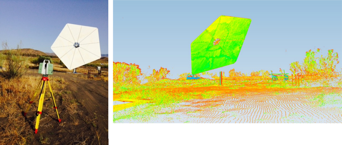
Photogrammetric shape and deformation measurement of heliostats
Close-range photogrammetry (PG) can be used to derive absolute shape and relative deformation if the PG is repeated for the same object studied under different conditions (elevation angles, altering the effect of dead load). This is especially useful for deformation studies for heliostats at different elevation angles. The following example illustrates the photogrammetric measurement of shape and deformation of a 40 m2 heliostat at the CESA-1 heliostat field at the Plataforma Solar de Almería, Spain.
Prior to the measurement, the heliostat had been equipped with 216 retroreflective targets (18 targets on each mirror panel), a measurement cross with coded targets of known dimensions, and one or two scaling bars (here: one) with precise knowledge of the distance between all the scaling bar targets. Fig. 5.6 shows the heliostat with the photographer on top of a lifting platform.

The heliostat has been positioned in nine orientations with the elevation being between 0 degrees (vertical) and 90 degrees (horizontal). In each orientation, one photogrammetric measurement has been performed, comprising 20 photos of different positions around the heliostat. The RMS measurement uncertainty was estimated to be below 0.1–0.7 mm, depending on the heliostat orientation. Especially for vertical orientations of the heliostat, there are restrictions concerning the camera positioning. Fig. 5.7 shows a photographic shot of the scene with bright reflecting targets. The right of Fig. 5.7 is a close-up of the scaling bar which is fixed on the right upper border of the heliostat.

The photogrammetric measurement results in a three-dimensional point cloud. Subtracting the ideal geometry from the measured points after appropriate spatial transformation, the deviation from the ideal shape is obtained.
Alternatively, using the three-dimensional point cloud and triangulation, the real surface normal vectors are calculated and can be compared with the normal vectors of the ideal shape. Surface slope deviations to the ideal shape can be calculated for each normal vector.
Deformation studies of a prototype heliostat, for example, show how stiff a heliostat is and in which way it deflects under gravity load in the different heliostat orientations. For this reason, the point cloud of a photogrammetric measurement in one elevation is subtracted from a point cloud of another elevation after the two point clouds have been superimposed. The result for the deflections in z-direction (the heliostat normal) after the heliostat has been moved from an almost vertical elevation (10 degrees) to a horizontal elevation (90 degrees) is shown in Fig. 5.8. We easily recognize that the heliostat edges deflect most strongly, with values of up to almost 5.5 mm. The corners that are furthest away from the heliostat center sag. The mean deflection normal to the aperture of the heliostat is 1.85 mm.

Heliostat shape characterization with laser radar
Alternatively to photogrammetric techniques, laser scanners can be used to derive 3D data of a heliostat. Fig. 5.9 shows the measurement setup to determine the heliostat shape using a laser scanner and a result.
Deflectometric measurement system for heliostat fields
Deflectometric measurement systems are perfectly suitable to derive slope information of all reflective surfaces like mirrors or glass surfaces. The measurement procedure is fast and accurate. If the distance between heliostat and target is very large, the target has to be larger or the measurement has to be taken in various steps and the pictures have to be assembled later on.
The basic measurement approach for a central receiver plant is shown in Fig. 5.10; see also Ulmer et al. [12]. A beamer projects a series of horizontal and vertical stripe patterns with sinusoidal brightness variations on a screen or directly on the tower. The heliostats have to be oriented in a way, so that the reflected pattern is visible in the photos. The camera takes automatically pictures of one or several heliostats; see Fig. 5.11.


Prior to evaluation, the camera, heliostat and target position have to be explored. The task is to determine the vectors r and i, i.e., to identify unambiguously the point on the heliostat and the corresponding point on the projection screen. The heliostat normal vector n can then be calculated by:

Once the surface normal vectors are known, the ideal normal vectors can be subtracted and hence the slope deviations of the heliostat can be determined.
As the fine stripe patterns shown in Fig. 5.11 on the right-hand side do not allow a unique assignment of the stripes, the measurement procedure is started with the projection stripes with large wavelengths as shown on the left, thus consecutively allowing a unique identification on the target.
Fig. 5.12 shows the slope deviations as results of a deflectometric measurement. In contrast to a photogrammetric measurement, the high spatial resolution also allows the detection of deviations with smaller extent, for example, local deformations due to forces and moments introduced by the facet back structure. There is less noise visible in the image compared to the photogrammetric technique. The figures on each facet are mean values of the slope deviations, indicating the alignment of facets on the heliostat structure (canting). The heliostat has a lower focal length than its ideal shape, because the slope deviations in x-direction on the left-hand side are positive values, while on the right side, they are negative. The RMS over the whole heliostat slope deviations is a measure for the quality of the heliostat shape. The RMS value of the heliostat shown in Fig. 5.12 is 1.98 mrad.

Using a pan-tilt-head mounted digital camera and wireless communication technologies, the measurement can be made highly automated. Commercial systems are available in the market to measure the slope deviations of whole plants in one night.
The deflectometric method allows the derivation of slope deviations in a fast, automated, and accurate way for whole heliostat fields. However, defined by the positions of camera, target, and heliostat, the heliostats can only be measured in one orientation. Hence, to characterize the deformations due to gravity, PG is a good standard method. Combining a deflectometric dataset for the heliostat shape and photogrammetric data for the deformation in different elevations due to gravity is recommended to ensure a comprehensive optical assessment.
These datasets can be used to simulate accurately the solar flux distribution of a single heliostat by raytracing. If all the heliostat orientations of the whole solar field are known, the flux distribution of the solar field on the receiver aperture can also be predicted with high accuracy.
Heliostat beam characterization and tracking error by flux measurement
The heliostat can also be characterized by a heliostat beam characterization system (BCS), comprised of a charged coupled device (CCD) camera and a white target, on which the heliostat is focused (Fig. 5.13). Two types of parameters can be derived by these images of the solar focus. The first parameter is the total beam dispersion error, which includes heliostat errors like canting and contour errors, mirror roughness, and loads like gravity temperature, and wind. This parameter also includes effects like astigmatism and meteorological parameters such as sunshape and scattering on the light path. To get the heliostat beam quality, astigmatism and the effect of sunshape and scattering have to be subtracted.

The second parameter of interest for a heliostat is its tracking accuracy. Taking a series of photos of a heliostat image on a white target, the tracking accuracy can be measured. In addition to the tracking offset, a possible drift of the solar beam over the day can be determined (see also Chapter 1, Fig. 1.9). Taking photos with a high frequency, the effect of wind and the effect of the controller logic can be assessed.
Flux density measurement on receiver aperture plane by moving bar
Heliostat shape information, their deformation with gravity, temperature, etc., and the tracking behavior under wind determine the optical performance of a heliostat. The overlay of all single heliostat beams of the whole solar field results in the solar focus on a receiver aperture. The useful part of the solar focus enters into the receiver aperture, and generally a smaller part is lost as spillage. Generally, receivers are sensible to high peaks of solar flux. For these reasons, the solar flux distribution in the receiver aperture is essential. The flux distribution represents the performance of the heliostat field if meteorological effects like sunshape and extinction are neglected. The flux distribution integrated over the aperture is the solar power entering the receiver which can be defined as acceptance criterion for a heliostat field at specific testing conditions (position of heliostat, receiver, and sun, atmospheric conditions like atmospheric extinction and influence of sunshape).
Different systems to measure the solar flux distribution exist; see Röger et al. [34]. The state-of the-art methods are presented here; new methods that are still under development are presented in Chapter 7.
The most commonly used indirect method uses a white diffusely reflecting moving bar target, a radiometer, and digital camera. The camera is either a CCD type or complementary metal-oxide-semiconductor (CMOS) type. It records the flux brightness distribution reflected off the white target. This measurement principle has been used since the end of the 1970s worldwide in different R&D central receiver projects; see for example Thalhammer [35], Neumann and Monterreal [36], and Lüpfert et al. [37]. In the case that there is no large Lambertian target, a moving bar is often used to scan the whole focal area while a camera takes several photos (e.g., the ProHERMES system at the Plataforma Solar de Almería (PSA) [37]); see Fig. 5.14. After image acquisition and deskewing, the target region is cropped in each image and combined to a surface covering the whole region of interest. The resulting image is corrected for camera nonlinearities, dark current, and shading, and is finally calibrated by a radiometer. Due to aging and soiling of the white reflective target and radiometer, a periodic recalibration must be foreseen. The ProHERMES moving bar has been working without mechanical problems. Having corrected systematic uncertainties, Ulmer [38] and Ulmer et al. [39] report a low total measurement uncertainty of solar flux density, being in the range from −4.7% to +4.1%. A total error of about 6% is reported for the BCS, being the calibration uncertainty of the flux gauge the principal source of uncertainty (5%) [40]. Ulmer [38] also identifies the flux gauge calibration as the highest contribution and assumes the error to be about ±3%.

The direct methods use sensors which are either mounted on a moving bar (see Chapter 7) or which are stationary and distributed over the receiver aperture. Moving parts are avoided if several water-cooled flux gauges are distributed in the aperture plane or on the receiver surface. Heat flux maps can be created by interpolation between the measurement points. Numerous sensors are required to obtain accurate results. Nonequal sensor distribution over the measurement surface allows the reduction of the sensor number while maintaining a reasonable measurement uncertainty. Stationary sensors were used, for example, at the PS-10 plant in Seville [41]. Measurement accuracy at sensor locations is high; however, spatial resolution may only be moderate while not using excessive numbers of sensors. Maintaining the reliable operation of high numbers of sensors in high-flux high-temperature receiver zones over the lifetime of a receiver is a challenging task. Experience has shown that the lifetime of flux gauges in the receiver environment may only be about 6 months [42].
Sensors like the most commonly used Gardon-type radiometers must be calibrated to measure the solar flux directly or to be used for calibration of brightness maps provided by digital cameras. This is because the manufacturer's calibration method differs in the spectral composition and angles of incidence from the solar use. Experience of an international comparison campaign between different solar flux gauges in a solar furnace using Kendall or calorimetric radiometers as reference are reported in Kaluza and Neumann [43]. A calibration method that uses the Gardon sensor as calorimeter by measuring inlet and outlet cooling water temperatures is presented in Ballestrín et al. [44]. As an electrically heated furnace is used, the calibration constants are corrected to be used with solar radiation. The achieved measurement uncertainties are estimated to be in the range of 2% [44].
5.2.3.2 Parabolic trough collectors
In order to compare several independent methods, selected PTCs at the PSA have been characterized with deflectometry, PG, and other methods.
Object preparation and image acquisition for the PG is similar to the photogrammetric measurement of a heliostat. It can be useful to apply the PG directly to the structure with dismantled mirrors, in order to distinguish effects arising from the metal structure from effects created by the mirrors.
For the measurement of the absorber position, either PG or manual measurement of the glass envelope tube can be applied, followed by estimation of the eccentricity of the steel absorber tube relative to the glass envelope tube. For this purpose, digital images are semiautomatically evaluated. These images are taken along the optical axis and perpendicular to the optical axis and vertex. The edges of the steel and glass tube are calculated from a cross section perpendicular to the focal line (see Fig. 5.15).

The TARMES approach (deflectometry) described in Section 5.2.2.1 is often applied to parabolic troughs to derive slope deviation data in high spatial resolution. The absorber tube position is an important input for the TARMES measurement and for a subsequent raytracing analysis. Typical mirror slope deviations obtained with the TARMES method and an intercept map are presented in Fig. 5.16.

5.3 Performance assessment of power and energy
5.3.1 Solar power plant performance characteristics
Parabolic trough power plants consist of large fields of mirrored PTCs, a heat transfer fluid (HTF)/steam generation system, a power system such as a steam turbine/generator cycle, and optional thermal storage and/or fossil-fired backup systems. Solar tower systems use a heliostat (reflector) field directing the sun's rays to a receiver (heat exchanger) on a high central tower. The working fluid in the tower receiver can be molten salt, water/steam, air, CO2, or other suitable fluids, each with their own particular attributes.
As noted in Section 5.1.1, these plants are being constructed in capacities of several hundred MW, resulting in very large solar fields. That section also introduced the issues associated with the variable solar input and its influence on the thermal equilibrium of performance testing. Consider, for example, a field of PTCs or a power tower heliostat-receiver combination. As the sun moves across the sky, the effective energy into the receiver varies with time of day, latitude, and weather. To achieve a suitable performance test, attention has to be paid to the nature and magnitude of this variation, and periods selected (typically tens of minutes) when the input energy is appropriately steady to achieve acceptable test results. Transients that are too high can result in test uncertainties outside a desirable range.
In large solar fields such as those noted above, there can also be spatial variations due to fluctuations in cloud cover that can impact the results. Clear sky testing is always preferable, but if this is not possible due to the season or time constraints, then the expected impact on test uncertainties should be examined prior to testing.
5.3.1.1 Illustration of input energy variations by season and time of day
Consider a parabolic trough system oriented on a north–south direction, tracking east to west. The useful or effective energy input to a trough collector is the vector of the solar direct radiation perpendicular to the aperture, which is termed ANI and calculated from:
where ANI is the aperture normal insolation (W/m2), DNI is the direct normal insolation (W/m2), and θ is the incidence angle of the direct normal radiation relative to the collector aperture plane.
The incident angle depends on the location of the plant (longitude and latitude), time of the day and the year, and orientation of the collector. Several algorithms are available to calculate the sun position and angles (see, e.g., Blanc and Wald [45] and Reda and Andreas [46]).
Consequently, the characteristics of the ANI are dependent on the weather, location, day of year, time of day, and collector orientation. Fig. 5.17 shows the variation of ANI at a good solar site in a western United States location from the period 08:00 to 16:00 for Jun., Mar., and Dec. A similar plot for DNI would show a much stronger variation. It can be seen that the ANI is quite steady during midday in both Jun. and Mar., and quite high in Dec.

A more important characteristic is the magnitude of the change in ANI during a test period. Fig. 5.18 shows the percentage changes in ANI over the previous 30 minutes during the daytime hours for these 3 months. It can be seen clearly that the variations between 09:30 and 15:30 in Jun. and Mar. are reasonably small. Such results could be used to identify suitable test periods with small variations in ANI.

5.3.1.2 Impact of variations on solar thermal and electricity test results
Variations in the solar resource affect both the solar system thermal tests and the power block electrical output tests. For the former, the measured output quantity is the energy input to the HTF. The HTF then flows to the steam generator trains to produce input steam for the turbine. Variations in the input steam conditions, particularly flow rate, will have a significant influence on the steady-state condition of the electricity output. Therefore, standard test procedures for conventional power plants cannot be applied and new procedures have to be defined that take into account the variable nature of thermal energy and electricity supply.
However, there are two important exceptions to this “rule”: plants with thermal storage and plants with auxiliary fossil firing. Consider the most straightforward thermal storage configuration, namely a tower system with a molten salt flowing through the receiver and then into a large hot molten salt storage tank at high temperature. Hot molten salt is drawn from the hot storage tank and passes through the steam generator complex to generate turbine inlet steam. In this case, the variations in weather are fully compensated by the buffering of the hot storage tank, and the steam production is isolated from the solar resource variations. The case of a plant with auxiliary fossil-fired boiler are even simpler in this aspect, for when these boilers are used—for example, during a week of inclement weather—the electrical output is steady due to a steady fossil fuel input.
5.3.2 Overview of typical tests
Characteristics and testing of individual components have already been described in Part 1 of this book. The tests of the individual components can generally be performed in the workshop or in a laboratory, whereas the tests described in this chapter refer to larger subsystems and complete systems. Due to the size, this equipment can only be assembled on site. Therefore, it is specific to utility-scale CSP system tests that they are being carried out on the installed system.
Typical tests of solar plants can be distinguished according two main criteria:
• Which part of the system is tested?
• What is the duration of the tests?
The plant systems of interest for performance testing are:
• thermal performance of the solar system; and
• electrical performance of the complete plant.
Accordingly, the complete system can be divided into two major subsystems: the solar system and the power cycle. The power cycle is a standard turbine cycle very similar to that used in conventional power plants. All operating commercial power plants currently implemented for utility-scale solar plants utilize Rankine steam cycle systems. In future, gas turbine cycles and dish Stirling engine systems may be of interest. This chapter is based on state-of-the-art steam cycle plants.
The main difference between a solar and a conventional power plant is that the fossil-fired boiler of a conventional plant is replaced by the solar boiler, which then will provide the heat input for driving the steam cycles. Therefore, an independent test of the thermal performance of the solar boiler as a major subsystem is important and sometimes conducted in commercial projects. Relevant thermal assessment methods are covered in Sections 5.3.4 and 5.3.5.
The assessment of the electrical performance of the complete system is, of course, of main interest for a commercial acceptance of a solar power plant. Corresponding tests are discussed in Section 5.3.6.
With regard to test duration, two main sets of tests are recommended:
• short-term steady-state tests; and
• multiday production tests.
The objective of the short-term steady-state test is to evaluate and verify the output, capacity, and/or efficiency of a plant or subsystem at certain ambient conditions. The ambient conditions are mainly solar radiation, ambient temperature, humidity, wind speed and direction, including the time of day and specific date because the sun position depends on these parameters. For the short-term tests, solar radiation and other conditions should be stable or vary only in a relatively small range so that the resulting output, capacity, and/or efficiency also varies only in a small range. Since solar input by nature varies continuously, the time span for these tests is relatively short. Depending on the allowable variation, it ranges from several minutes to ~2 h. Typically, steady-state test results can only be achieved under clear-sky conditions.
Tests at full load may be conducted to demonstrate the full capacity of the plant at certain ambient conditions. Power output and capacity tests can be at full load or at the output/capacity possible at the available weather conditions. The test output may be referenced to a performance model (see Section 5.3.3) or another calculation or procedure agreed upon by the testing parties.
Short-term steady-state tests are not sufficient to demonstrate that the plant is able to achieve the expected energy production over time. Several factors influence this observation, including:
• steady-state conditions are difficult to reach over a longer period; and
• operation of the plant is very often at part-load conditions and/or under transient operation conditions.
Therefore, continuous multiday production tests are often conducted for purposes of demonstrating long-term energy generation. During these tests, the total energy production measured over the course of a multiple-day period is determined. The output is then referenced to a performance model. The objective of these tests is to verify that the system is able to produce the output projected by the performance model. The minimum duration is recommended to be at least 10 days, but may last as long as one complete year. During the multiday production test, different weather and operation conditions will be covered, and start-up and shutdown processes will be included as well as other intermittent and stop/start conditions. Ten operation days may represent sufficient different operating conditions.
5.3.3 Application of performance model
In order to evaluate the test results, the measurements must be compared against expected results. Due to the complexity of the solar system and the variable nature of the solar resource, it is necessary for valid results to calculate the expected output by means of a validated solar system computer performance model. Such models calculate the performance of a solar power plant based on given input conditions, like solar radiation and other appropriate weather conditions. In addition, plant status parameters, such as availability of collectors and heliostats or reflectivity of mirrors, can be considered as inputs. A computer model has the advantage of taking into account all performance factors simultaneously. Therefore, such a model is better able to predict performance results for a large variety of different combinations of parameter and conditions that are changing continuously and that might be different than the set and sequence of parameters and conditions used for the design of the plant.
For test evaluation purposes, the model calculates the plant performance based on the actual weather conditions and plant status parameters agreed upon by the test parties. The actual data should be perfectly synchronized in time with the measured test data. Based on these inputs the expected thermal power, electrical output, or efficiency for the test period will be calculated by the model. Once the predicted performance is computed, it can be compared to the corresponding as-tested values. The measured results must, of course, take into account the uncertainty interval for each measured value. The uncertainty band for the result should always be given in the test results. Uncertainty is discussed further in Section 5.3.5.4.
For steady-state conditions (i.e., the short-term tests) and when certain boundary conditions, such as incident angle and/or collector/heliostat position, are limited, a set of correction curves may be considered to calculate the expected performance instead of a computer model. However, due to the higher accuracy and complexity of the input factors, the use of computer models is highly recommended.
5.3.4 Description of tests
5.3.4.1 Short-term steady-state tests
The purpose of this test is to measure the thermal or electrical power output and/or efficiency of the solar system over a short period at steady-state conditions. Since perfect steady-state conditions are difficult to achieve even for a short period, acceptable stability criteria have to be defined for the following variables:
• minimum level and maximum allowable variation of DNI;
• maximum allowable variation of mass flow;
• maximum allowable wind speed;
• level and variation of inlet and outlet temperature and, if appropriate, pressure;
• reflector cleanliness at or higher than a specified minimum level; and
• availability of collectors/heliostats at a minimum level.
Uncertainty analyses on the test results (discussed later) will provide quantitative insights on the allowable variations in the individual measurement components. Prior to starting the tests, the plant must be operated for a sufficient period of time (stabilization period) under steady-state conditions as defined above (e.g., 0.5–1 hours). If measurements have to be interrupted because stability criteria were violated, the tests have to be repeated, including the stabilization period. Typically, test duration ranges from 15 minutes up to 2 hours or more.
Four types of tests should be considered for the short-term test needs:
1. Design/full power capacity test: During this test the thermal power output of the solar field and/or the electrical output of the total plant will be measured. The objective of this test is to verify that the plant and all related components and subsystems, e.g., HTF pumps and collector field or power block, are able to deliver the full design power output. Minimum solar conditions may be defined for this test.
2. Power test at available conditions: While the full power test requires high radiation conditions in order to achieve full output, this test can be performed at lower solar radiation, expanding the range of possible test days. During this test the thermal and/electrical power is measured. This test does not have to be conducted at full capacity; in fact, one objective of this test is to verify the power output at less-than-design capacity conditions. The measured output is to be compared with an expected output calculated using the solar system performance model.
3. Outlet temperature test: The objective of this test is to demonstrate that the solar system is able to achieve its design temperature at the outlet. For the solar power tower plant the solar system definition includes the receiver. Thermal power tests and outlet temperature tests should be performed at the same time.
4. Efficiency test: For the efficiency tests, the same test results as for the power tests can be used, but the solar conversion efficiency at the available test conditions shall be calculated from the measured result. Corresponding equations are provided in Sections 5.3.5.2 and 5.3.6.2. The measured value can then be compared with the expected value calculated using the performance model.
5.3.4.2 Multiday production test
The objective of the multiday production test is to measure and evaluate the solar system total thermal energy production and/or the plant total electricity production over a longer period. Thus, different operating conditions are evaluated such as start-up and shutdown, part load operation, and transient conditions, which all contribute to the overall energy production at different performance levels. Both clear sky and partly cloudy conditions are acceptable. The result of the tests is to be expressed as a direct measurement of total energy production during the test period. The test period should be long enough to contain sufficient representative days. A period of at least 10 days of continuous operation is recommended, though longer periods are preferable, e.g., 30 days. The measured results are to be compared to the same values as calculated by a performance model for the same period.
The primary objective of this test is to run the test continuously without any interruption for the complete period. However, if a relatively short period for the duration was selected, e.g., 10 days, minimum requirements for the solar radiation need to be defined. Days that do not meet this requirement have to be excluded and the test has to be extended until the required number of days with acceptable conditions has been accumulated. For some commercial plants, debt providers have required one full year of successful operation at design conditions.
5.3.5 Solar system performance
5.3.5.1 Description of boundaries of the solar system
As with any performance test, test boundaries need to be defined. The solar system is comprised of the solar reflectors, solar receiver, and heat exchangers needed to transfer the collected solar energy to the working fluid of the power block. An example of the solar system boundary is shown in Fig. 5.19 wherein the inputs are the solar resource, inlet working fluid, internal solar system parasitic power,1 and, if required, auxiliary heating. The sole output is the increase in enthalpy of the working fluid.

In the case of a parabolic trough system, the solar system includes the PTCs, all piping that connects the individual collectors with each other, and the piping required to transport the working fluid from the system boundaries to the collectors and back to the system boundaries. Usually it also includes the pumping station for the working fluid and other equipment required to handle the working fluid, like the expansion vessel and fluid conditioning system.
In the case of tower systems, the solar systems includes the heliostat field, the power tower receiver and all piping and equipment that is required to transport the fluid from the system boundary to the receiver and back to the system boundary. Configurations with water/steam and air working fluids are direct systems in which heat is added directly in the receiver to the working fluid of the power cycle. In an indirect system such as a molten salt configuration, heat is added to a molten-salt HTF in the receiver and subsequently transferred to the power-cycle working fluid in a steam generator train. The steam generation train may be inside or outside the test boundaries.
The appropriate test boundary locations for the measurement of thermal performance should be chosen by the test parties based on the equipment configurations and test requirements. The scope of this chapter does not include a thermal energy storage system, nor co-firing with a natural gas boiler within the test boundary but focuses on the solar boiler only.
To be clear, the term solar field is used in the case of parabolic trough technology for the array of PTCs connected to each other. In the case of a tower plant, the solar field is comprised of an array of heliostats.
5.3.5.2 Solar system thermal calculations
The primary objectives of the thermal assessment are to determine the following thermal performance values:
• outlet temperature;
• thermal efficiency; and
• thermal energy output within a specific period.
Thermal power output
The thermal power of the solar system is determined from the increase in enthalpy flow between the inlet and outlet of the system. A cold fluid is sent from the power block to the solar system. There it is heated up to the desired temperatures. The thermal output can be calculated from:
where Pth is the calculated thermal power output (kW), ![]() is the mass flow rate of HTF (kg/s), hHTF,out is the enthalpy of HTF out of the system (kJ/kg), and hHTF,in is the enthalpy of HTF into the system (kJ/kg).
is the mass flow rate of HTF (kg/s), hHTF,out is the enthalpy of HTF out of the system (kJ/kg), and hHTF,in is the enthalpy of HTF into the system (kJ/kg).
Usually several data will be taken in defined time intervals and an average value for the thermal power will be calculated:

where n is the number of measuring events.
The enthalpy of a fluid depends on the temperature and the pressure. In the case where the HTF is water/steam or air, values for the enthalpy can be taken from general tables such as steam tables, when temperature and pressure are known. In the case of other HTF, like thermal oil or salt, corresponding tables should either be provided by the supplier or enthalpy values have to be determined by laboratory measurements. The uncertainty of the calculation for Pth, however, will be strongly influenced by the uncertainty in the enthalpy values.
Outlet temperature
The outlet temperature is of major importance since it directly affects the efficiency of the power cycle. The temperature can be measured with appropriate instruments (see Section 5.3.5.3) and average values can be calculated as follows:

where TOut is the outlet temperature (K).
Thermal efficiency
The thermal efficiency is the efficiency of the conversion of solar radiation into thermal energy by the solar system. It can be calculated from:

where ηth is the thermal efficiency of solar system (%) and Aaperture is the solar field aperture area (m2).2
For a number n of measuring events, the average efficiency is calculated as follows:

Eq. (5.8) can generally be applied to both parabolic trough and solar tower systems. However, for parabolic trough systems, the efficiency is often referred not to the DNI but only to the component of the DNI that is normal to the aperture plane of the collector, the ANI (for the definition of ANI, see Section 5.3.1):

In carrying out the tests described above, a variety of details and component-level decisions must be established. For example, the following considerations may be required:
• inclusion, or not, of gaps between reflector panels in a solar field in the computation of total reflector area;
• similarly, the handling of tracking collectors during a test in which solar conditions and/or outlet temperature control require changes in the number of collectors during a test run; and
• proper accounting of broken reflectors or receiver tubes in the solar field during a test run.
Thermal energy output
Since load conditions of a solar power plant vary over the time of the day, for the multiday performance test the thermal energy output is of interest. The thermal energy output can by calculated by integrating the power output (Eq. 5.4) over the corresponding time period. The formula to obtain the thermal output (or thermal production) is then computed from:

where Qsolar is the calculated thermal capacity delivered by the field (kWh) and Δti is the time interval between data measurements (s).
5.3.5.3 Instruments
The primary measurements needed to calculate the performance values of Section 5.3.5.2 are the:
• temperature at the inlet and the outlet of the solar system as defined by the system boundary;
• mass flow at inlet and outlet of the solar system;
• pressure at inlet and outlet of the solar system; and
• direct normal irradiance (DNI).
In addition, the following measurements should be performed since they are used as an input to the performance model:
• wind speed and direction; and
• mirror reflectance.
It is not the purpose of this book to provide a complete treatise on standard measurement techniques. Those can be found in relevant codes and standards like the ASME performance test codes (PTCs). Rather, a comprehensive overview of applicable instruments will be given and some specific information on solar-unique measurements will be provided.
Accuracy and measurement uncertainty always play an important role in performance measurements. Due to the nature of variability of the solar recourse and the imperfections of the control system, this is of particular importance for solar thermal power plants. Therefore, Section 5.3.5.4 will specifically discuss measurement uncertainties.
Temperature
For temperature measurements, standard resistance temperature detectors (RTDs) or thermocouples (TCs) can be used. The higher accuracy of the RTDs suggests it is better suited for acceptance testing. RTDs are available at different accuracy levels. For acceptance testing, a platinum 4-wire sensor with high accuracy should be chosen, e.g., Class A according to DIN ICE 751. It is strongly recommended, or required by test codes, to calibrate the individual devices used during performance measurements. The calibration should be performed with the primary element including the transmitter or even end-to-end (i.e., sensor-to-display). The temperature sensor should be immersed in the fluid. ASME PTC 19.2 recommends that the immersion length should be at least 75 mm, but not less than one-quarter of the pipe diameter. For accurate performance measurement, the installation of redundant devices is required. For additional information, ASME PTC 19.2 provides more details on temperature measurement.
Flow meters
Most flow meters actually measure the velocity of the flow or a pressure difference. Knowing the detailed geometry of the pipe and the measurement device as well as the fluid properties, the volume and mass flow are computed. In order to determine the fluid properties, the temperature and pressure have to be known. The required measurement instruments are often directly included in the flow measurement device.
ASME PTC 19.5 provides information on different flow measurement devices. The selection of the device, of course, depends on the HTF used in the solar system. In the case of water-steam as HTF, standard devices used in steam power plants are appropriate (see PTC 19.5).
Most commercial parabolic trough power plants use synthetic oil as HTF. According to PTC 19.5, a number of flow measurements are suitable. In practice, usage in several commercial solar trough plants has tended towards ultrasonic and vortex flow meters. Installation instructions provided by the supplier shall be followed. For flow measurement it is specifically important that the device is located in a fully developed flow that is not disturbed by fittings or other pipe fixtures. The required minimum upstream and downstream straight pipe length without disturbances depends on the measurement device and the pipe diameter.
Pressure measurement
For pressure measurements, standard pressure transmitters can be used.
Direct normal irradiance
The accurate measurement of direct normal irradiance (DNI) is of major significance since this value presents the heat input into the system and is, therefore, analogous to the fuel input in a conventional thermal power plant. Generally, there are two different ways to measure the DNI. It can be measured directly by a 2-axis tracking pyrheliometer. These devices use either a thermoelectric or photoelectric detector for converting solar flux (W/m2) into a proportional electrical signal [47]. The use of view-limiting apertures inside a pyrheliometer allows for the detection of only normal (or almost normal) incoming radiation, requiring that this instrument be mounted on a 2-axis tracker in order to follow the sun continuously.
The second option is to use one or more pyranometers. This device uses a similar detector to that of a pyrheliometer, but the incoming radiation is not restricted by any kind of apertures. Therefore it does not only measure the incoming direct normal radiation, but also the global radiation, which is made up of direct and diffuse radiation. If such a detector is shaded by a so-called shadow band, the direct normal radiation is filtered and only the diffuse radiation is detected by the sensor. Combining the information on global and diffuse measurement signals, the direct normal irradiance can be computed.
Since the pyrheliometer has a significantly higher accuracy than the pyranometer (according to Stoffel et al. [47] the expanded uncertainty of the pyrheliometer is 2.4% instead of 4.8% for the pyranometer), only the first device is recommended for performance measurements.
For an accurate performance measurement, at least two DNI instruments with high accuracy are required. In practice, for large solar fields and for purposes of the short-term tests additional instruments placed at different locations across the solar field are often used. For long-term tests and normal operation, the short-term impact of DNI fluctuations due to locally restricted cloud coverage becomes less significant and redundant measurements at fewer locations in the solar field may be sufficient.
More details on radiation measurements can be found in Chapter 2.
Wind speed and direction
Wind speed and direction measurement are not necessary to measure the thermal performance of a solar system. Some performance models use this information as an input to calculate possible impact on the optical accuracy of the collector and the heliostat. However, this effect is relatively small for moderate wind speeds. The wind speed is mainly used to determine if actual conditions do not violate test or operating conditions. At high wind speeds, collectors or heliostats need to be put to a safe position in order to withstand the high wind loads. Typical maximum wind speeds are in the order of 13 m/s. On the other hand, low wind speeds are recommended for short-term performance tests to ensure that there is no effect of the wind on the optical accuracy. A typical boundary for this speed is 7 m/s. However, these limits may change with technology.
Consequently, wind speed and direction are only secondary parameters, and accuracy of measurement is of minor importance. Standard cup anemometers for wind speed and wind vanes for wind direction can be used. Measurements shall be taken at 10 m height and therefore devices shall be mounted on a mast.
Mirror reflectance
Reflectance is typically measured with a specular reflectometer. The reflectance of the solar mirror has a direct and strong impact on thermal performance, as 1% of reduction in reflectance leads to almost 1% of reduction in efficiency. Therefore, reflectance of the mirror (or reflector) is another important input parameter to the performance model. It is a characteristic of the mirror itself and can be measured in the laboratory (compare Chapter 3). However, in the field, mirror reflectance is affected by soiling. Therefore, it is essential to characterize the actual reflector cleanliness during performance tests in order to determine accurately the expected performance at the actual conditions. Since this is not easily done in large utility-scale solar fields, the approach used in this regard must be agreed upon by the test parties.
Reflector cleanliness is determined by measuring the reflectance of a mirror in the field and comparing the result with the reflectance of a clean mirror.

In order to improve the accuracy, it is essential to do both measurements with the same device and at the same spot.
It should be noted that reflectance depends on the wavelength of the incoming radiation and on the selected acceptance angle (specularity). In contrast to laboratory measurements, field measurement devices do not measure the reflectance across the complete solar spectrum, but only at a single wavelength. Therefore it is important that this single measurement is done at a wavelength with high solar irradiance, such as the range between 500 and 700 nm.
Reflectance values also depend on the acceptance angle of the measurement device. Acceptance angle requirements vary with the focal length of a system. A longer focal length results in a lower acceptance angle. State-of-the-art field reflectance measurement devices can be adjusted to different acceptance angles. Therefore, especially for PTCs, the selected acceptance angle of the field measurement device should fit to the acceptance angle of the collector. For solar towers, the focal length varies strongly across the field with the distance between heliostats and tower. In this case, an average acceptance of the measurement device should be selected.
Soiling rates of mirrors may depend on the specific location in the field. For example, mirror panels that are close to the ground usually experience a higher soiling than those mirror panels at a higher position. In addition, locations at nearby roads or cooling towers are known for higher soiling rates. Therefore, measurements should be done at a representative number and location of mirrors distributed uniformly and randomly across the complete solar field.
The measurement device, the number of measurements taken and the procedure to be applied must be selected and documented carefully for a representative performance test.
Data acquisition
All data, except the reflectivity measurements, should be collected and recorded by an automatic data acquisition system. Sampling interval should be at least every 5 seconds. For the short-term tests, the data should be stored at that sampling rate. For long-term tests, one average value per minute can be calculated and stored in order to reduce the number of stored data.
Reflectance measurements will be collected by a portable measurement device and data will be recorded manually. A data collection sheet should be prepared that identifies the test site location, date, time, data point position, and type of data collected.
5.3.5.4 Measurement uncertainty in solar system testing
Due to various influences, any test result will have an associated uncertainty. The uncertainty interval around a measured result describes our lack of knowledge about the true value of a measured quantity. Uncertainty can be reduced by many repeated measurements and in some instances can be further reduced through the use of redundant instruments.3 The uncertainty of an interval about a measured value is usually expressed with a probability or level of confidence. Uncertainties arise from possibilities for error arising from or classified as: systematic errors, random errors, and human errors. It is very important in the measurements discussed here to quantify the uncertainty intervals to make judgments on the validity of the test results.
Test uncertainty is a very important element within Performance Test Codes, such as those published by the ASME in the United States, which has placed critical importance on test uncertainty analyses of all measurements and calculations associated with PTCs. ASME PTC 19.1—Test Uncertainty is devoted to this topic, and plays an important role in all ASME PTC codes. The text in this section is extracted for illustration from a recent NREL report [48] on solar system acceptance test guidelines.
Because of the resource variability and imperfections in control systems, variation in all of the measured parameters is inevitable. The frequency and period of data collection directly impacts the test uncertainty, and it is highly recommended that a pretest uncertainty analysis be carried out prior to selection and subsequent installation of any instrumentation. A solar power test will typically consist of more than one test run (data collected during a period of time in which the measured parameters are relatively steady). Conducting more than one test in addition to a post-test uncertainty analysis is recommended to verify the repeatability of the test results and the validity of the pre-test uncertainty analysis.
The systematic error associated with a measurement of a single parameter can come from many sources, including the calibration process, instrument systematic errors, transducer errors, and fixed errors of method. The test engineer should be diligent in identifying all of these sources of error, although it is often the case that one or several will dominate within a particular measurement parameter.
Random errors can similarly be based on a manufacturer's specification. However, the random uncertainty for a given measurement can be reduced based on repeated measurements over the interval in which the system is considered to be in thermal equilibrium (defined by a minimal change in the DNI plus working fluid flow control over the test period, such that the effects of thermal exchange between the working fluid and the receiver hardware are negligible). For repeated measurements, the random standard uncertainty can be defined by:
where SX is the standard deviation of a series of sampled data and N is the number of data points collected over the test interval (e.g., 180 data points for a 30-minute test with data collected at 10-second intervals).
The essence of an example calculation is described below using the ASME PTC 19.1 principles and notation (compare also Ref. [49]). The purpose is to describe how the uncertainties in each of the measured variables X associated with an acceptance test propagate into the value of a calculated resulting quantity R.
Calculated results, such as the delivered power and the solar thermal efficiency, are not typically measured directly, but rather are based on parameters measured during the course of one or multiple tests. For this case, the result, R, is a function of individual or average values of these independent parameters as described by
where the subscript i describes the number of parameters used in the calculation of the result and ![]() is either the value of a single measurement of the parameter or the average value of the parameter based on a number of N repeated measurements.
is either the value of a single measurement of the parameter or the average value of the parameter based on a number of N repeated measurements.
The expression for the combined standard measurement uncertainty of a calculated result based on multiple error sources can in many cases be calculated from the root sum square of the total uncertainty of the individual systematic and random error sources4:

where bR is the systematic standard uncertainty of a result and SR is the standard random uncertainty of a result as calculated by


For the equations above, ![]() is defined as the systematic standard uncertainty5 of a component and
is defined as the systematic standard uncertainty5 of a component and ![]() is the random standard uncertainty of the mean of N measurements. Definitions for the standard systematic and random uncertainty, as well as the methodology for calculating these values, are described in detail in PTC 19.1 and Dieck [49].
is the random standard uncertainty of the mean of N measurements. Definitions for the standard systematic and random uncertainty, as well as the methodology for calculating these values, are described in detail in PTC 19.1 and Dieck [49].
The total standard measured uncertainty of the calculated result given by Eq. (5.13) can be calculated using the methodology described above. It is important to note that this “standard” uncertainty implies that the calculated result will capture the true result within a 68% confidence level (one standard deviation). Typically, a confidence level of 95% (two standard deviations) is desired by the testing parties. For this case, the expanded uncertainty in the result is given by
A detailed application of this method for both the solar system thermal power output and solar system efficiency can be found in the NREL work [48] for the cases of a parabolic trough system and a molten salt power tower system, respectively. Using reasonable values for the test parameters, representative uncertainties were calculated. Although any such analysis must be undertaken with the specific system and instrumentation in mind, the systematic and random uncertainties of measurement parameters calculated in the treatment represent what may occur in a typical field installation. Actual uncertainties depend on specific field instrumentation and calibration procedures associated with an acceptance test.
For a 100 MWe solar tower power plant with 6 hours of thermal storage, the results in that case were in the order of 3.2% and 4.1% for the solar field thermal power and thermal efficiency, respectively. For the trough plant, the results were 3.9% and 4.7%, respectively.
5.3.5.5 Example of thermal efficiency results
Fig. 5.20 gives an example of results for the measured thermal efficiency at a clear day for a state-of-the-art PTC (for details, see Ref. [51]) operated in a commercial power plant. The values are calculated based on Eq. (5.8) using measured values for temperature, flow, and DNI. Each dot represents a 10-min average value. The graph shows typical values for the efficiency and a characteristic shape of the curve over the day. The values are rising steep in the morning and falling steep in the evening due to shading effects of adjacent collectors. The typical dip during noon is caused by the incident angle effects. The error bars representing the mean uncertainty of the results are also shown.

Fig. 5.21 illustrates the effect of the incident angle on the collector efficiency based on measurements performed within different periods of the year. The abscissa shows the absolute values for the incident angle. It can be clearly seen that thermal collector efficiency is worse during winter than during summer, which is mainly caused by the higher incident angles in the winter period.

5.3.6 Total plant performance
5.3.6.1 Description of system boundaries
The assessment of the performance of a utility scale solar plant is tied to the warranty/guarantee agreements between the technology suppliers and financing parties. A typical scenario is that the plant is designed and constructed by an EPC company under contract to the owners. The EPC provides the guarantees for the performance based on the successful completion of specified performance tests. A crucial element of the EPC contract is the definition of the elements, requirements, and timing of those tests. A number of test definitions are possible, usually a function of the perceived risks in solar system performance.
Section 5.3.5 discusses acceptance tests of the solar system, which usually fulfill one element of the total EPC performance test requirements. In practice, the EPC contract with the owners is usually based on the electrical output of the total solar power plant, while testing of the solar system performance itself is carried out to satisfy contractual agreements between the EPC contractor and the solar system supplier.
The total plant includes the solar system, power block, and balance of plant, as well as ancillary systems such as thermal storage and fossil fuel co-firing. A schematic for a parabolic trough system including all these subsystems is shown in Fig. 5.22 (compare also Ref. [54]). Test boundaries for the total plant performance will include all these subsystems. The inputs into the system are:

• auxiliary fossil heat; and
• parasitic power for in-plant needs, that is, the difference between gross and net electrical output,
while the output is:
• gross electrical power at the generator; and
• net electrical power to the electrical grid.
5.3.6.2 Calculations
Following the test approach presented in Section 5.3.4, the following values will be either directly measured or calculated from the measurement result:
• gross and net electrical power output Pel (MW)
• solar-to-electric efficiency
• electric energy output within a specific period Eel (MWh).
Gross and net electrical power output Pel
The electrical power measurements for gross and net electrical output would normally be done at the terminals of the generator and at the transformer station, respectively. Depending on the purpose of the test and the agreements between the testing parties, the power of the electrical consumers within the plant, such as pumps, fans, HVAC, etc., may need to be monitored in the performance assessment.

where Pel,net is the net electric power (MW), Pel,gen is the gross electric power at generator (MW), and Pel,con,i is the parasitic power of in-plant consumers i (MW).
Solar-to-electric efficiency ηel
The solar-to-electric efficiency is the efficiency of the conversion of solar radiation into electric energy by the solar system. It can be calculated from

For a number n of measuring events, the average efficiency is calculated as follows:

Eq. (5.19) is generally applied to both parabolic trough and solar tower systems. However, for parabolic trough systems, the efficiency may also be referred to the ANI rather than the DNI:
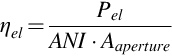
In the case of a solar power plant with fossil co-firing, the test either should be performed without using fossil heat input or it is required to consider the fuel contribution in the calculation. For that purpose the so-called solar share (SS) is introduced. The solar share defines the ratio of the electricity produced by the sun in relation to the total produced electricity:

Looking at the electric output, it is difficult to determine which contribution is coming from the sun and which from the fossil firing. Therefore, very often the solar share is calculated based on the thermal input into the system

where QFuel is the thermal input delivered by the fossil fuel (kWh).
Considering now the solar share according to Eq. (5.21), the solar-to-electric efficiency for a solar power plant with co-firing can be calculated as follows:

For plants with integrated thermal storage, also the loading status of the storage at the beginning and the end of the test must be considered:
where ΔQTES is the difference of loading status of thermal energy storage (kWh), QTES,start is the loading status of thermal energy storage at the beginning of test period (kWh), and QTES,end is the loading status of thermal energy storage at the end of test period (kWh).
With this, the thermal energy storage share TS can be defined:

Eq. (5.24) assumes that the storage system is not within the boundary of the solar system as defined in Section 5.3.5.1.
Considering Eq. (5.24), the solar-to-electric efficiency for a solar power plant with thermal storage can be calculated as follows:

Electric energy output Eel
The electric energy output can by calculated by integrating the power output Pel over the corresponding time period. The formula to get the electric output (or production) is then computed from

5.3.6.3 Conduction and evaluation of tests
The concept of thermal equilibrium for short-term testing is of equal importance in the measurement of total plant electrical output and solar system thermal output. Therefore, the performance test procedures laid out in Section 5.3.4 (short-term steady-state tests and multiday production tests) are also applicable for electrical performance.
As no solar-oriented test codes are available for overall plant performance at present, more general test codes must help to fill that gap.
ASME PTC 46, described below, is one of several good choices to fill that need. The test results from the use of PTC 46 would be compared to a projection of electrical output based on the test conditions using a sophisticated total plant performance model as discussed in Section 5.3.3. Other than the stability of steam flow and conditions into the steam turbine, there are in general terms no solar-specific aspects to electrical output testing.
Typically, ASME performance test codes address tests of short duration (measured in minutes, not hours, days, or longer) with constant energy sources. For a solar power plant with a Rankine cycle steam power block, the EPC contract will typically include a requirement to demonstrate the warranted electrical power output in MWe. But, in contrast to a fossil-fired plant, there will also be a requirement for the solar power plant to show the actual energy generation over time in kW-hours compared to that projected by the plant performance model based on actual solar radiation conditions and contractual parameters for power block and solar system characteristics. The time period may be for several months or even up to 1 year.
For the assessment of the total plant performance, the performance model has to consider, in addition to the inputs discussed in Section 5.3.3, the input of fossil fuel during the test and the loading status of the thermal storage system at the beginning and the end of the test.
For the long duration energy generation test, there will be no requirement related to test uncertainty because test conditions will normally not be steady and equipment conditions can vary widely, e.g., the mirror reflectance over a large solar field.
5.3.6.4 Example plant performance data
Typical electrical performance data for large utility-scale solar plants are shown in Table 5.1. These values are representative for plants in high solar resource regions (e.g., southwest United States, South Africa, Morocco) and thermal storage in the 6–10 full-load hour range.

5.3.6.5 Electrical test considerations
The crucial solar-related impact on a standard test of the steam turbine power block is the stability of inlet steam to the turbine. Other than that, the performance testing of the power block is well covered in available test codes.
For the short-term test, the steam turbine cycle output can be measured in a thermally stable condition if the solar steam input is acceptably steady, as mentioned above.
ASME PTC 46 (see Section 5.3.7.3), as an example, also stipulates a significant number of other code requirements to ensure valid results, providing useful and extensive details. In concert with that code, ASME PTC 19.1 gives tight requirements on the uncertainty measurements.
For illustration, the following paragraphs show a few general comments on the requirements of PTC 46 for understanding the electrical side of solar plant performance tests. Note that all aspects of procedures, equipment, measurement, uncertainty, and other factors are covered in that code. For actual testing with valid results, the full stipulations of that code must be adhered to rigorously and in depth.
The primary objective is to obtain test results with a very low measurement uncertainty for specific test requirements defined to achieve that objective.
Examples of those requirements include:
• complete records of the testing, including equipment, configuration, valve line-up, instrumentation, data acquisition, test procedures, test logs, and test data;
• for all instruments: type, model, purpose, location, redundancy, and calibration records;
• detailed test plan and test procedures, including stabilization criteria, number and duration of test runs, requirements for initial equipment conditions, including solar field reflector reflectivity;
• performance model for comparison to measurements agreed upon by test parties;
• uncertainty analysis using ASME PTC 19.1, both pretest and for all test results; and
• criteria for acceptance/rejection of individual test results.
5.3.7 Codes and standards
Currently, there are no published international standards available that deal with plant performance assessment of CSP systems. Two committees have been formed to close this gap: one by the American Society of Mechanical Engineers (ASME) and one by the International Electrotechnical Commission (IEC). As of early 2016, no standards have been published by either group. Below, a brief description of the scope of the codes is provided.
In order to bridge the period until official standards are available, the National Renewable Energy Laboratory (NREL) of the U.S. Department of Energy initiated the development of Performance Test “Guidelines” that were published in 2011–13.
The Spanish Association for Standardisation and Certification (AENOR) has developed a national standard that covers performance tests for parabolic trough power plants. The code, published in 2015, is described in Section 5.3.7.2.
5.3.7.1 NREL performance acceptance guidelines
Lacking published international standards or codes for performance testing of utility scale solar thermal systems, NREL6 undertook in 2009 and 2013 the publication of “Guidelines” to provide direction for conducting performance acceptance testing for large parabolic trough [48] and power tower [48] solar systems that could yield results of a high level of accuracy consistent with good engineering knowledge and practice. The recommendations in those Guidelines were reviewed by stakeholders representing concerned organizations and interests throughout the CSP community. The Guidelines recommend certain methods, instrumentation, equipment operating requirements, and calculation methods. The primary objective of the Guidelines was that, when tests are run in accordance with the methodologies, the test results would yield a valid indication of the actual performance of the tested equipment. It is important to note that the Guidelines are only recommendations—to be considered carefully by the contractual parties involved in the acceptance testing—and it is likely that modifications would be required to fit the particular characteristics of a specific project.
Notably, the Guidelines do not specify means to compare test results to contractual guarantees. A key presumption is that the parties to a commercial test will address that issue, as well as agree on other important issues with regard to testing protocol and evaluation of test results. The approach taken in the Guidelines is that the measured test results will be compared to projections from a performance model based on the measured meteorological conditions and agreed-upon solar system characteristics.
The scope of the solar system discussed in the NREL Guidelines does not include a thermal energy storage (TES) system. However, even if the scope did include a TES system, the methods of testing the solar field/HTF system itself would be similar, if not identical, to the guidance given in the Guidelines. A separate set of tests and objectives would be required for TES system acceptance.
5.3.7.2 AENOR UNE 206010
In Apr. 2015, AENOR published the Spanish standard on tests for verifying the performance of solar thermal power plants with cylindrical PTC technology (Spanish original title: “Ensayos para la determinación de las prestaciones de las centrales termosolares con tecnología de captadores cilindroparabólicos”).7
The standard is applicable to solar thermal power plants of any size with parabolic-trough collectors, with the sun as main source of energy, optional non-solar energy sources, and an optional thermal storage system. It does not include any other CSP technology, such as solar towers.
The code is intended to be applicable to acceptance testing in such power plants, or other scenario in which their performance must be known and thus will help in identifying possible operational problems that are affecting output.
The evaluation of the test requires:
1. use of a plant simulation model that can generate reference values when the input conditions measured during testing are entered; and
2. a defined verification procedure, a way in which measurements and uncertainties are to be compared to the reference values from the plant simulation model.
Similar to the NREL performance acceptance guidelines, two types of tests are proposed, a short- and a long-duration test:
1. Short-duration testing (at least 24 hours): the purpose is to verify the performance of the power plant over a short period of time during clear days, including a full charge-discharge cycle of the thermal storage if available, recommended to be performed three times. DNI>700 W/m2 must be available for at least 4 hours, recommended without auxiliary heat source.
2. Long-duration testing (at least 365 days): the purpose is to verify or validate annual plant production and auxiliary consumptions (electricity and non-solar fuel).
The tests combine measurement and comparison to a predefined simulation model for the following operation parameters:
• available solar radiation (DNI);
• plant electric consumptions;
• net electric generation (high voltage side of transformer);
• non-solar energy, backup fuel; and
• net plant efficiency.
The test definitions are based on practical experience with commissioning and acceptance testing of many of the Spanish parabolic trough plants that came online between 2009 and 2013.
The English version of the text is also the basis for the corresponding IEC TC117 (see Section 5.3.7.5) international working group from 2016 onwards.
5.3.7.3 ASME PTC 52
In 2009, the American Society of Mechanical Engineers (ASME) formed a committee to develop a Performance Test Code (PTC) for concentration solar power systems. The code will provide procedures for conducting tests and analyses to determine the performance of CSP plants such as in parabolic trough, continuous linear Fresnel reflector and power tower technologies. ASME PTC-52 is intended to cover the solar-to-thermal conversion system only and not the complete power plant. The solar-to-thermal conversion system, i.e., the solar system or solar field, is treated as one component as a part of the whole power plant similar to a conventional boiler or to a steam turbine generator that are covered under different ASME performance test codes. As such, ASME PTC-52 will cover some aspects discussed in this chapter.
In accordance with the current practice that is described in the NREL performance acceptance guidelines and that is also discussed here, PTC-52 proposes to conduct short-term tests as well as multi-day tests. The code also elaborates the use of a performance model to evaluate the tests and to establish the expected output against which the actual test output will be compared. Details on test procedures, instruments and methods for measurements, calculation and reporting of measurement results, as well as on uncertainty analysis, will be given in the code. It will additionally contain a short digression on thermal storage.
When complete, PTC 52 is expected to supplant need for the NREL guidelines. The issue of the first version of PTC-52 is planned for 2017.
5.3.7.4 ASME PTC 46
The ASME Performance Test Code 46 (PTC 46) entitled “Overall Plant Performance” is internationally respected and often used for overall plant performance testing. As stated in the introduction to the Code, the objective of PTC 46 is to provide uniform test methods and procedures for the determination of the thermal performance and electrical output of heat-cycle electric power plants at a steady-state condition over a few hours, and provides explicit procedures for the determination of the following performance results: corrected net power, corrected heat rate or efficiency, and corrected heat input. Test results provide a measure of the performance of a power plant or thermal island at a specified cycle configuration, operating disposition and/or fixed power level, and at a unique set of base reference conditions.
Due to the thermal stability requirement of PTC 46, only the short-term solar system testing discussed in earlier sections strictly fits into this dictate, though many of the specific code requirements are applicable to the longer multi-day tests as well, as can be seen in the following paragraphs.
Test results can then be used as defined by a contract for the basis of determination of fulfillment of contract guarantees. Test results can also be used for comparison to a design number, to trend performance changes over time, to help evaluate possible modifications or to validate them, or for any application in which the overall plant performance is needed.
5.3.7.5 IEC TC 117
The International Electrotechnical Commission (IEC) is currently developing a standard for CSP plants (IEC TC 117)8 that is not restricted to the solar-to-heat conversion system like the ASME PTC 52, but rather intends to cover the complete solar power plant for the conversion of solar radiation into electrical energy. When completed, this standard would not only cover the plant in total but will discuss all elements (including all subsystems and components) of the entire power plant. It will include all of the current different types of systems, as parabolic trough, solar tower, linear Fresnel, dish, and thermal storage. The standard would not only address performance measurement and test methods, but also design, installation and safety requirements, as well as power quality issues. The section of the code that covers total plant performance testing will be based on the Spanish standard UNE 206010 (see Section 5.3.7.2) and will probably not be published before 2018.
5.3.7.6 Other codes
Several other codes are available that cover performance aspects of solar thermal collectors as a component, such as the International Standard ISO 9806, the European Standard UNE-EN 12975-2 and the American Standard ASHRAE 93 and ASTM E 905-87. These standards cover explicitly or can be transferred to concentrating and tracking solar thermal collectors and, therefore, can be applied in principle to parabolic trough and linear Fresnel collectors.
However, these standards do not cover complete large-scale systems and cannot be applied to the systems described in this chapter. Some of the tests and measurements described in the standards mentioned above can be used to derive collector parameters that can be used as an input into the performance model.
5.4 Outlook
As discussed earlier, the tests described in this chapter require either steady-state conditions in short-term tests or a multi-day test period in non steady-state conditions. However, steady-state conditions cannot be predetermined since they depend mainly on the weather and, therefore, time periods that fulfill these requirements are limited. Further, the testing period in terms of the multi-day test is relatively long compared to other acceptance test requirements in the power industry. In order to overcome these restrictions, new test approaches are being considered that allow achieving comprehensive performance information in a shorter time period. Chapter 7 discusses several new approaches that are currently under investigation.