10. Mapping Data
A map does not just chart, it unlocks and formulates meaning; it forms bridges between here and there, between disparate ideas that we did not know were previously connected.
—Reif Larsen, The Selected Works of T. S. Spivet
In a broad sense of the word, this entire book is about maps, as it deals with the spatial representation of information with the goal of revealing the unseen. In this chapter, I will be using a narrower meaning of “map” to refer just to visualizations that display attributes or variables over pictures of geographical areas.
As any of the other graphic forms we’ve learned about so far, maps can be used to communicate or to explore information. Maps are critical to many areas of inquiry, from epidemiology to climate science.
The main attributes of a map are its scale, its projection, and the symbols used to depict information.1 The scale is a measure of the proportion between distances and sizes on the map and those on the area represented—that is, how big is the map compared to reality?
1 In the next few pages, I will be following Mark Monmonier’s How to Lie With Maps (2nd ed., 1996.) For a complete list of books consulted, see the references at the end of this chapter.
There are many ways to express this ratio: as a verbal statement (“1 inch on this map represents 100 miles in the real world”); as a fraction (1:1,000, or, “One unit of measurement on the map is equivalent to 1,000 of those units in the real world”); or as a bar with a length that is equivalent to a rounded distance in reality (10, 100, 1,000 miles, etc.).
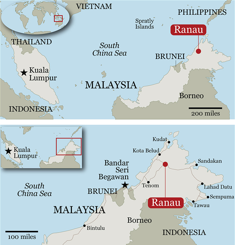
Maps can be classified according to their scale. A large-scale map (1:10,000, for example) will show a small area with higher detail than a small-scale map (1:100,000,000). When you represent Earth as a whole, you are using a small-scale map. A close-up of your hometown is a large-scale one.
The scale you choose for a map is closely related to your assumptions about how much most of your readers know about the area shown. A map like the first one on Figure 10.1, locating Ranau, in Malaysia, would be good for the International News section of a large American newspaper (therefore, the inset on the upper-left corner). The second map might be useful for South Asian readers, who are more familiar with these latitudes.
Projection
I don’t think that I’ll reveal anything new if I tell you that Earth is a globe.2 Transforming it into a two-dimensional representation is tricky. Imagine trying to wrap the peel of an orange over a flat surface without tearing it. That’s similar to what we need to do when we create a map.
2 Some people disagree. See http://www.tfes.org/, which isn’t a parody. These folks play on a higher league than those who still sustain that humans were created in their current form 6,000 years ago.
Projection is the process of making a globe, or a portion of it, fit into a flat picture. When you make that transformation, some features will always be distorted; some distances, shapes, and areas will be stretched, and others will be compressed. There’s no 100 percent accurate representation of a globe other than a globe itself.
As a visualization designer, it is unlikely that you will ever have to deal with the nightmarish math involved in the creation of projections, but you’ll often a) download copyright-free maps from the Internet to trace and modify, or b) generate maps with software tools like Geographic Information Systems (GIS). In both cases, it’ll be useful to get acquainted with some terms.
In technical jargon, the geometrical objects where the globe can be projected to create a map are called developable surfaces. The most widely used developable surfaces are the cylinder, the cone, and the plane. Figure 10.2 is an infographic that explains how elementary conical, planar, and cylindrical projections work.
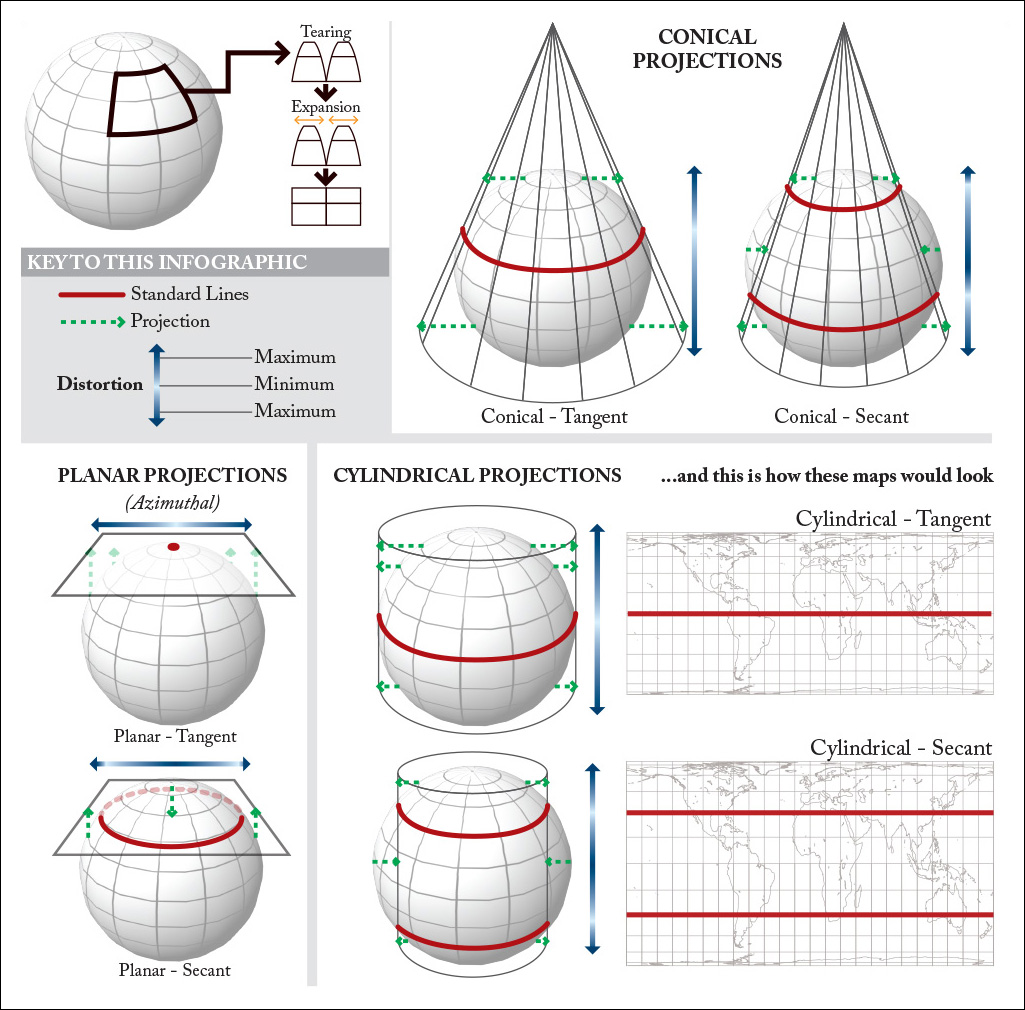
The areas of the developable surface that are tangent to the globe during the projection process are called standard lines. As a general rule, the scale of a map is only accurate along those lines. The farther away we move from them, the greater the distortion. As many mapping tools let you choose standard lines, it’s always a good idea to make sure that they are as close as possible to the area your story refers to.
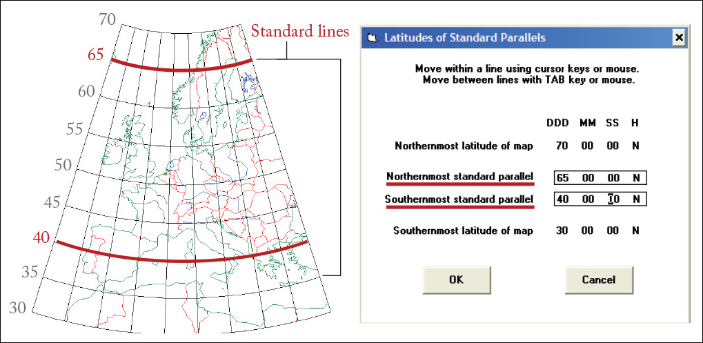
Figure 10.3 is a map of western Europe that I generated with an old free tool, Versamap. I chose a conical projection. Notice that the standard lines are the 65th and the 40th parallels north. Those two parallels nicely frame the region in which I’m interested.
There are five properties that can (and will) be distorted when you project a globe on a flat surface: shape, area, angles, distance, and direction. Any projection can respect one or two of those properties, but not more. At least three attributes will be sacrificed regardless of the projection you choose. Creating a flat map is always a trade-off.
Taking these properties as classifying criteria, we can identify two major map groups. Some maps preserve continental shapes—the overall look of landmasses—and local angles (any angle created by two intersecting lines will be the same on the map and on the globe). In software tools and cartography books, you’ll see that these are called conformal projections. The most famous one is the Mercator, the first one on Figure 10.4.
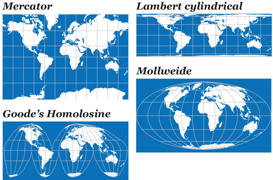
The Mercator projection was created for sea navigation, but it isn’t a good choice for world maps because landmass area ratios are totally off.3 As the standard line is placed on the Equator, the farther north or south you go, the larger the map regions will be in relation to reality. See Alaska, for instance, which looks as big as Brazil. It is a shame that the Mercator projection has become the standard in online tools like Google Maps.4
3 I like the Mercator projection, even if it’s so often misused. See Mark Monmonier’s Rhumb Lines and Map Wars: A Social History of the Mercator Projection (2004) for a forceful defense of it.
4 There’s a reason for this: Mercator is a good choice for maps of small areas, as it preserves shapes and angles. But it sucks when used on world maps. What could be the solution for online map services? Perhaps it could be switching projections depending on the region of the world readers are exploring and on how much they zoom in or out.
A second family of projections available in mapping software, equal-area projections, preserve area ratios. That is, the sizes of the areas represented on the map are proportional to the areas on the Earth. The Lambert cylindrical projection, also shown on Figure 10.4, is a good example. Equal-area projections tend to distort shapes heavily: the farther the distance from the standard lines is, the greater this distortion becomes.
No map can be conformal and equal-area simultaneously. Those are mutually exclusive characteristics. However, there are some projections, like Goode’s Homolosine, that are neither conformal, nor equal-area. They don’t respect shapes or sizes completely, but they achieve a reasonable balance between the two, and so are called trade-off, or compromise projections. The Mollweide projection is another example.
So the million dollar question is: how do I choose the best projection? I usually say about projections what Ellen Lupton wrote about choosing typefaces in her graceful book Thinking With Type (2004): there are no good or bad typefaces. There are appropriate and inappropriate typefaces. It’s the same for maps.
Imagine that you need to create a data map showing which areas of the world may be covered with ice for more than 90 percent of the year in 2020 (Figure 10.5). A Mercator projection would give you a different picture than a Goode map, as regions close to the poles look huge on the former and much smaller on the latter.
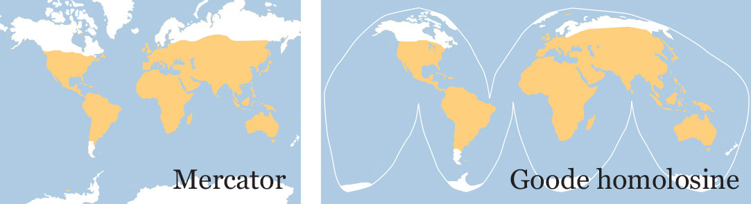
Figure 10.6 is a summary of very popular projections and of the cases when it is advisable to use them. If you are planning to show a larger region, a country, or even the whole world, it should be clear at this point that as a general rule you should always use a projection that preserves areas without distorting shapes heavily. If you are going to show just a very small region, such as your neighborhood or town, try to stick to comformal projections, those that preserve shapes and angles.
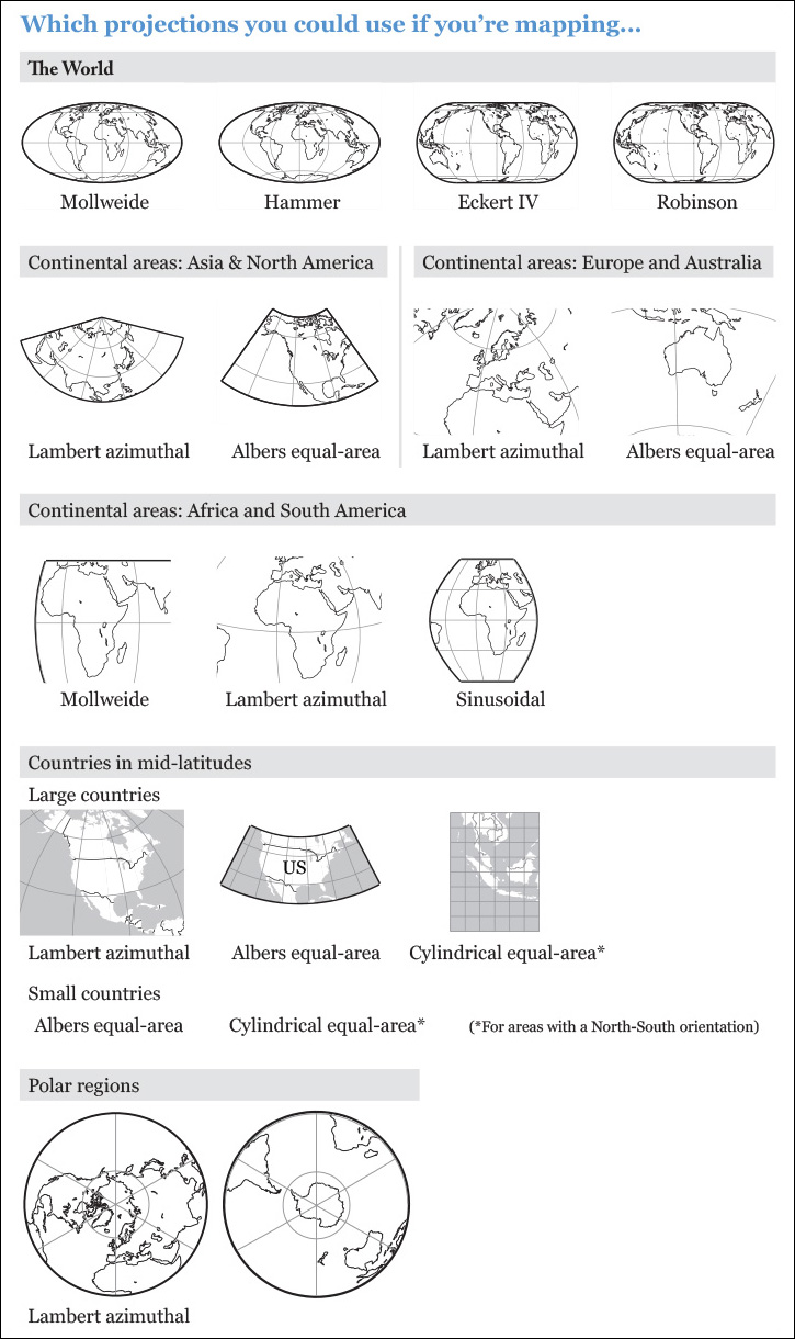
Figure 10.6 Projection suggestions. If you do maps for the Web, be aware that Mercator is the default projection many online tools use. Try to avoid it, using the recommendations above.
Playing with different projections can lead to beautiful visualizations. Back in 2012, John Nelson, a map designer, became interested in visualizing the paths of all hurricanes and tropical storms the National Oceanic and Atmospheric Administration has records for. Nelson first used some predictable projections (see one of his drafts on Figure 10.7). Then, he tried a projection centered on the South Pole, and the map became an unforgettable piece of art (Figure 10.8).

Figure 10.7 A draft for the map of hurricanes in Figure 10.8.
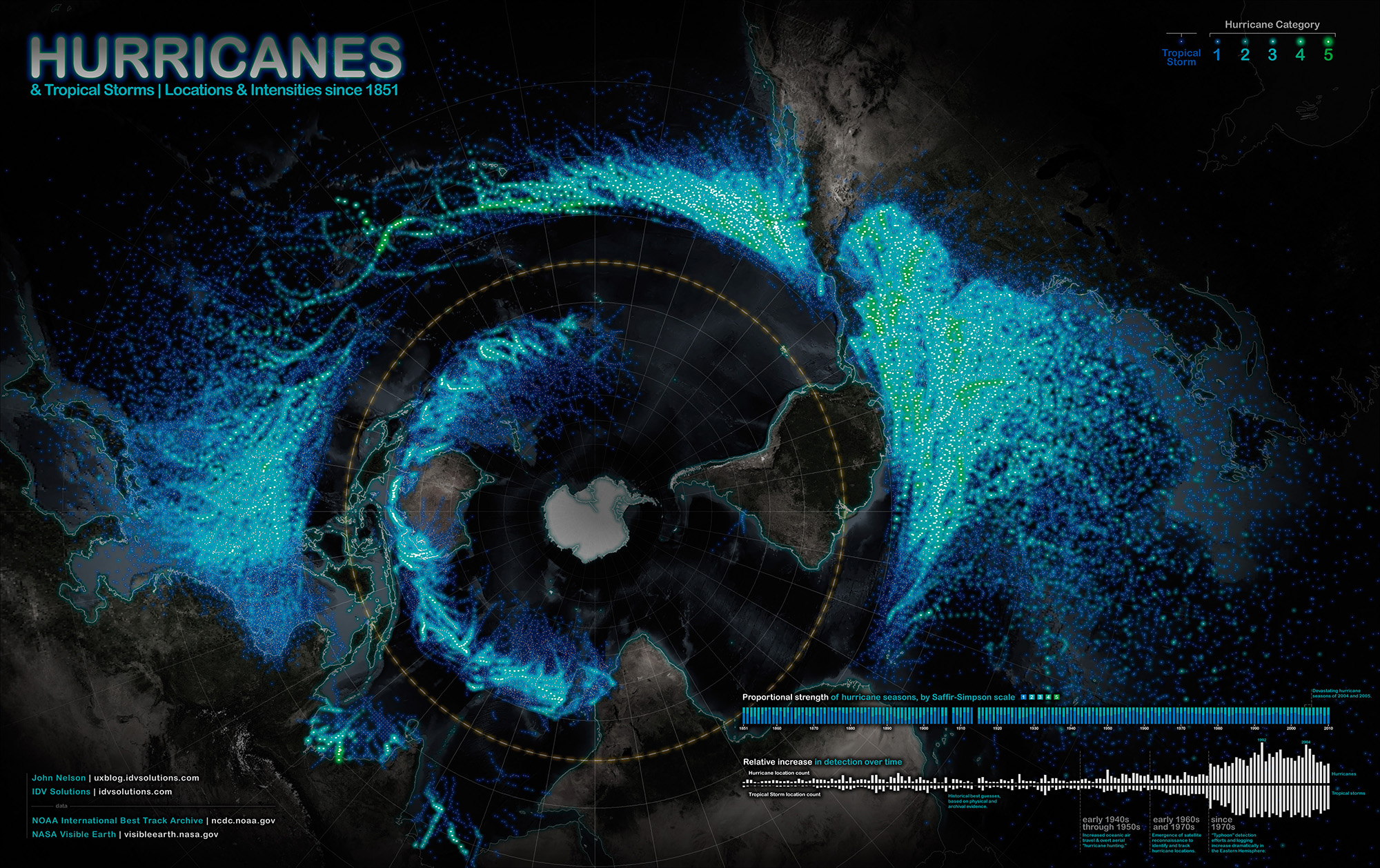
Figure 10.8 A map of hurricanes and tropical storms since 1851, by John Nelson: http://tinyurl.com/9y2axf4.
Data on Maps
In the literature about cartography, data maps are usually called thematic maps. Here’s the definition of thematic maps from Axis Maps, a cartography visualization firm: “Thematic maps are meant not simply to show locations, but rather to show attributes or statistics about places, spatial patterns of those attributes, and relationships between places.”5
5 Axis Maps has a good and free introduction to thematic maps: http://axismaps.github.io/thematic-cartography/articles/thematic.html.
Data on maps can be encoded by means of points, lines, areas, and volumes, as shown on Figure 10.9. Symbols can represent qualitative information (a location, the boundaries of an area) or quantitative information (magnitude or concentration of a variable or phenomenon in certain places).

Point Data Maps
The simplest way to put data on a map is by using dots representing either individuals or groups of a fixed size.
Figure 10.10 is a dot map of evergreen forests (green) and woody wetlands (blue). The data and the code behind this project comes from Nathan Yau, who regularly posts tutorials in his website (flowingdata.com) besides being the author of two books on data visualization. Each dot on the map doesn’t represent a single tree or plant—that would only be feasible if we were mapping a tiny area—but a spot of land that is mostly covered by each kind of vegetation.
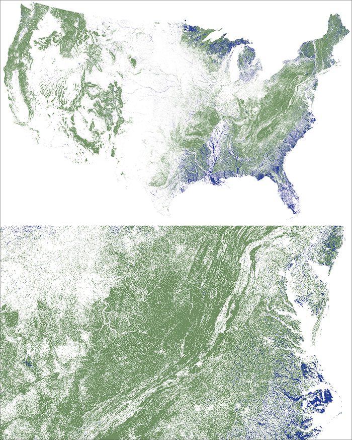
Figure 10.10 A dot map of evergreen forests (green) and woody wetlands (blue). The code used to create this map comes from www.flowingdata.com.
Another beautiful example of a dot map is Figure 10.11. This one was designed by The Baltimore Sun’s five-person design and development team, which is responsible for creating visualizations, apps, and infographics. Dots are color-coded according to race, so readers can immediately envision the segregation that ails Baltimore, which unfortunately also exists in many other U.S. cities.
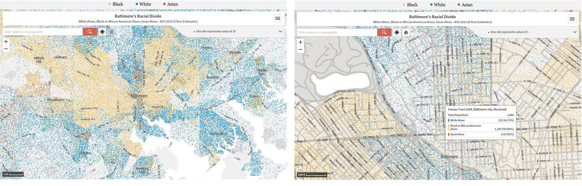
Figure 10.11 Legacy of segregation lingers in Baltimore, a dot map by The Baltimore Sun: http://tinyurl.com/osxj37x
On a dot map, quantity is represented by the amount and concentration of dots, but there’s another kind of point map that represents it through symbol size: the proportional symbol map. On a proportional symbol map, geometric objects (usually circles) or icons are scaled in proportion to quantitites. You can see an example on Figure 10.12, by The Washington Post.
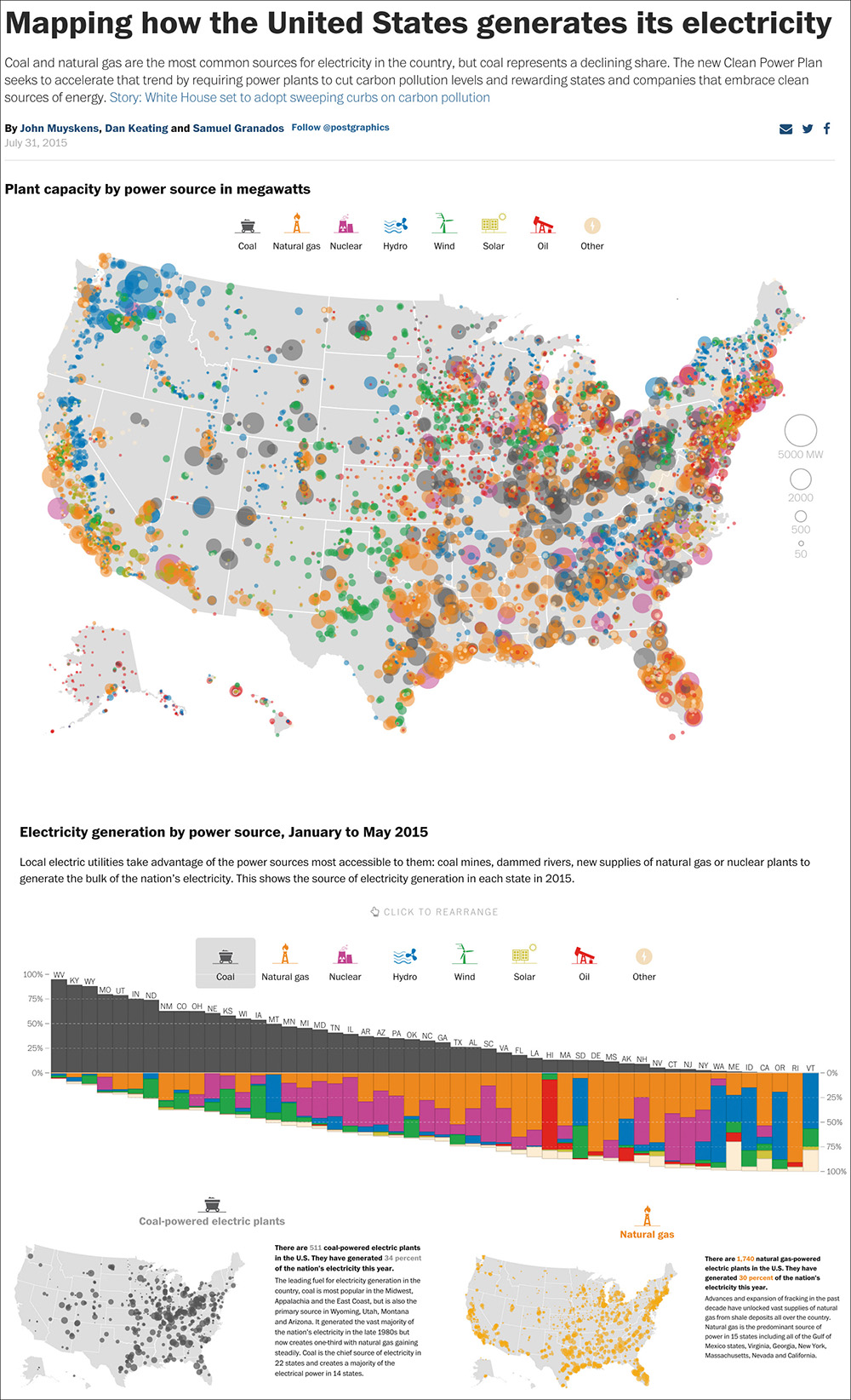
Figure 10.12 Proportional symbol maps and chart by The Washington Post https://www.washingtonpost.com/graphics/national/power-plants/.
There’s a lot to like in this project. The main map represents all energy plants in the United States The size of the circles is proportional to megawatts. A bar chart shows the percentage of energy generated in each state that comes from each source. This chart is sortable, so if you click on Nuclear, the bars will rearrange themselves: states getting most of their energy from nuclear plants will be placed on the left side. Finally, the designers were very aware of one of the main challenges in proportional symbol maps, the fact that excessive overlap may obscure information. Therefore, they added six smaller maps at the bottom, one for each power source.
Many visualization tools let you design proportional symbol maps quite easily, but there might be a case in which you’ll need to create them manually. Let’s suppose that we’re doing an income map with just three circles, corresponding to $100, $200, and $400. This should be easy, right? Just draw one circle to represent $100, duplicate it, and then scale it 200 percent to obtain the circle representing $200. The results are on the left side of Figure 10.13. They are horribly wrong.
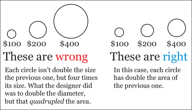
Just think about it: if you tell a software tool to scale something 200 percent, it will make it twice as tall and twice as wide. Therefore, you aren’t doubling the size of your original circle. You are making it four times larger. You can just eyeball the evidence for this: you can insert four $100 circles inside the area of the $200 circle, and four $200 circles inside the $400 circle.
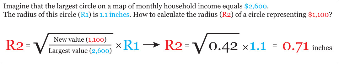
On the right side of Figure 10.13, circles are scaled correctly. How to size circles manually? Follow the formula on Figure 10.14.
This said, it’s worth remembering that maps are priceless at offering an overview of your data, but they don’t enable very accurate judgments. Even if objects on a proportional symbol map are correctly sized, readers won’t estimate their relative sizes well. Remember that area was on the lower half of the scale of methods of encoding (devised by William Cleveland and Robert McGill) that we saw in Chapter 5.
Cartographers often refer to phenomena like the Ebbinghaus illusion to illustrate maps’ shortcomings. An example of that illusion: If you surround two circles of the same size with larger or smaller circles, your perception of their size will change. (See Figure 10.15.)
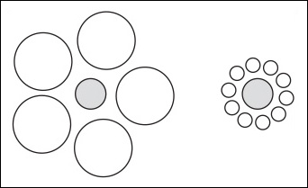
Figure 10.15 The Ebbinghaus illusion, named after German psychologist Hermann Ebbinghaus. The gray circle surrounded by large white circles looks smaller than the one surrounded by small white circles. In truth, they are the same size.
You also need to pay attention to symbol placement. Each symbol should be located where each value was observed. If the location is a point (a town, a city), this is quite easy: just center the symbol to the point. If the symbol represents a value associated with an area (a province, a state, a country), you should put it in the visual center of the region. There is an exception to this rule: when too much overlap occurs, it is acceptable to displace the symbols slightly off-center.
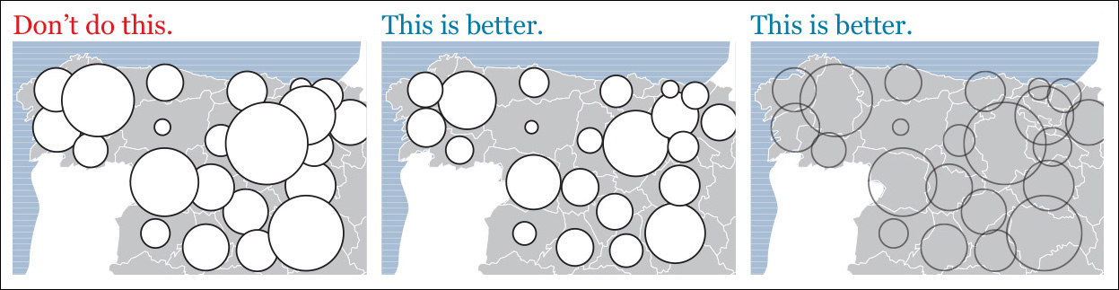
Overlaps can become problematic in proportional symbol maps: some areas may get so crowded that it becomes difficult to see what’s going on. There are two ways of addressing this problem, as shown on Figure 10.16: make sure that smaller symbols are always in front of larger ones, or make all symbols semi-transparent. If this is not enough to reduce clutter, scale all the symbols down.
Although there are no fixed rules about how to design the legend of a proportional symbol map, two main styles have become popular (Figure 10.17): nested (the smaller symbols are placed within the larger ones) and linear (the symbols are placed next to each other).

Linear legends can have a vertical or horizontal orientation. The number of circles on a legend depends on the amount of detail you estimate readers will need to understand the map. As a general rule, though, try not to use more than four.
The scores to include in the legend may vary depending on the content and goals of your map but, as a general rule, first include two circles representing rounded values that are as close as possible to the highest and lowest values in your data set. This will help readers get an idea of the range of your data set. After that, you can include a couple of extra circles proportional to rounded scores in between the highest and the lowest ones.
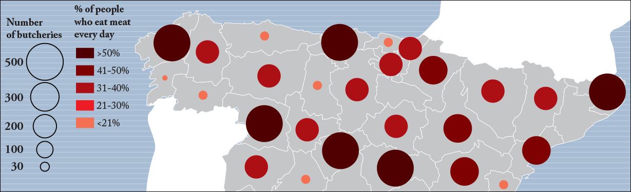
Proportional symbol maps can be multivariate. Simply using a second method of encoding (shading, for example, as in Figure 10.18) may give readers a more nuanced understanding of the data.
Line Maps
The most common kind of data map based on the use of lines is the flow map, usually showing the movement of entities between geographic areas.
Figure 10.19 was designed by Bestiario, a Spanish data visualization firm. It’s part of a huge project called “Commuting and Mobility Dynamics in the 73 Neighborhoods of Barcelona.” Based on data from mobile companies, Bestiario plotted several maps in which line weight is proportional to the amount of people moving from the neighborhood where they live to the places where they study or work.
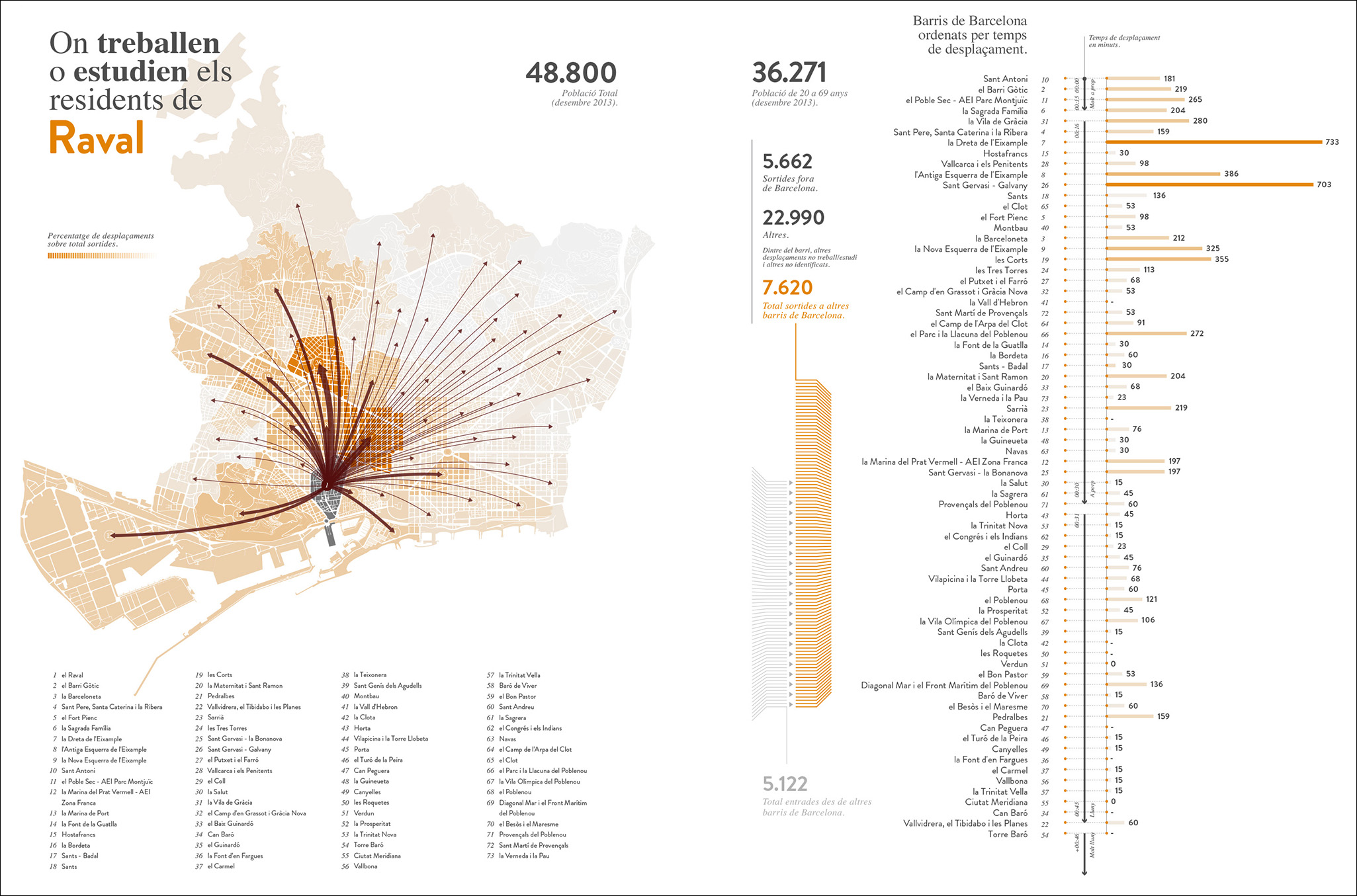
Figure 10.19 Graphic by Bestiario.org.
The maps are supplemented by bar charts on the right side. Here, neighborhoods are sorted according to how far they are from the point of origin. A black vertical line indicates time of commute. Bars are proportional to number of commuters.
The Basics of Choropleth Maps
A choropleth map encodes information by means of assigning shades of color to defined areas such as countries, provinces, states, counties, etc. A choropleth map can show different kinds of data (ordinal, interval, ratio, etc.), as Figure 10.20 shows.

Choropleth maps can be used for quick data exploration. Figure 10.21 is a set of maps that I put together recently to compare racial groups, per capita income, and median age in Florida.
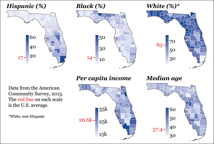
Figure 10.21 Exploring Florida with choropleth maps. Designed with code inspired by a tutorial by Ari Lamstein (www.arilamstein.com).
These maps are OK for what they are (letting me see interesting things in the data), but they have many flaws. To begin with, the three on top should perhaps share the same continuous color scheme. But I let the program choose this for me, forgetting my own dictum, never trust software defaults. (This is valid advice for any tool, not just for mapping programs.)
Sticking to software defaults uncritically will lead you to maps like Figure 10.22. Notice the color scales. In principle, they aren’t that bad: around 17 percent of the U.S. population is Hispanic, so these maps offer a quick “below average/above average” portrait. However, the fact that most values above the national average are grouped together exaggerates the amount of Hispanic people in the United States. To me, the county-level map suggests that in a large portion of the United States, more than half of the population is of Latino origin.
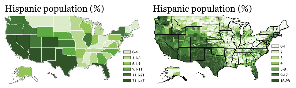
Figure 10.22 Two levels of data aggregation: state level and county level. If you paid attention to my words about projections at the beginning of this chapter, you may have noticed that these maps are based on a Web Mercator projection. That isn’t a great choice, but I couldn’t change the default projection in the software I was using!
In a choropleth map, each interval of values associated with a shade of color is called a class. Grouping values in classes in a way that causes relevant patterns to become visible without exaggerating them much is quite a challenging task, one that shouldn’t be left to a dumb algorithm to complete. Manual adjustments are often necessary.
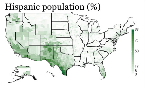
In the current county-level example, I’d like to use a scale in which the higher values are shown with more detail, something like 0–8, 8.1–17, 17.1–50, 50.1–75, and 75.1–98 (Figure 10.23). Notice that I put one break at 17 percent (the U.S. average) and another at 50 percent (beyond that, the majority of the population is Hispanic).
Classifying Data
Cartographers have developed multiple ways of choosing breaks and classes for choropleth maps. I’m going to explain how to design the most common ones. I’ll also show how to calculate them, even if in most cases your computer can do the math for you. When designing maps, always try different intervals until you find the one that better represents the data.
I’ll do this exercise using the percentage of Hispanic population at the state level. Figure 10.24 shows a strip plot in which each circle is a state, and a histogram of frequencies. Before you create any choropleth map, always take a look at the shape of your data, as we did in Chapters 6 and 7.
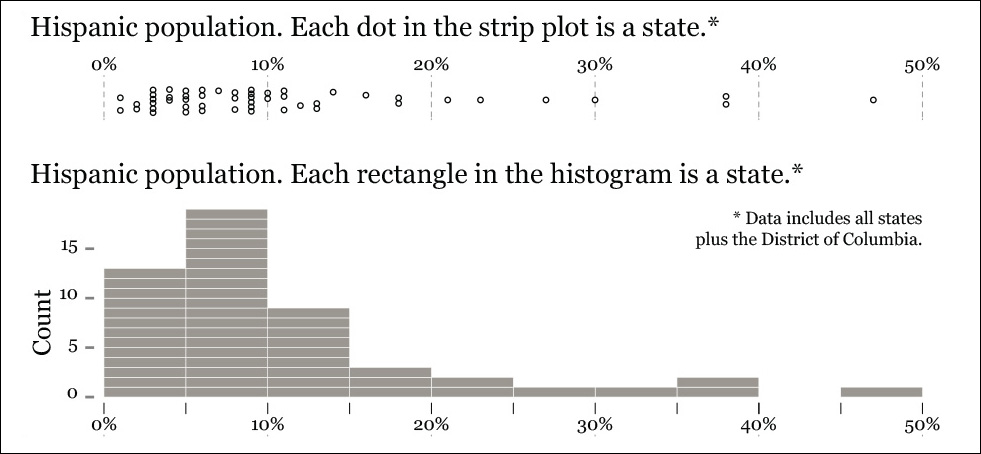
Our distribution is pretty skewed: nearly two-thirds of the states are on the lower end of the spectrum (between 0 and 10 percent); in only 17 of them, more than 10 percent of the population is of Hispanic origin. The minimum value in our data set is 1 percent (Maine and West Virginia) and the highest is 47 percent (New Mexico.)
The first method to calculate breaks is to place them at intervals of constant size. Boundaries calculated according to this method will enclose equal ranges of data, such as 0–10, 11–20, 21–30, 31–40, and so on. This method usually works well when frequencies are constant, but let’s give it a try. Here’s how to calculate your breaks:
Get the maximum and the minimum scores: 47 percent and 1 percent
Subtract them: 47-1 = 46
Divide the result by the number of classes (intervals) you want. Say you want 6:
46/6 = 7.7
This 7.7 is your class size. The lower boundary of your first class should be the minimum value, 1, and the upper boundary should be 8.7 (which is 1+7.7). The boundaries for the subsequent classes can be calculated just by adding 7.7 over and over again, as shown on Figure 10.25. For instance, the upper boundary of class two can be calculated with this formula:
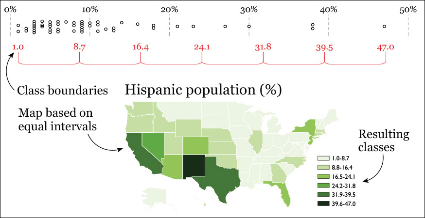
Minimum value + (2 × Class size); in other words: 1.0 + (2 × 7.7) = 16.4
The choropleth map based on equal intervals isn’t that bad, after all. New Mexico has a class of its own, and the states with the highest rates stand out nicely. But perhaps we are losing some important details at the lower end of the spectrum, as so many states lie within the 1.0 to 8.7 range. To reveal it, we may want to try something different.
Remember percentiles, explained in Chapter 7? We can use them to classify data, too. This is the quantiles method, and it consists on placing roughly the same number of cases (states, in the current example) inside each class. We have 51 observations in our data set, 50 states plus D.C., so we’d need to place roughly 51/6 = 8.5 states in each class. Some rounding and adjustment will be required. Notice that on Figure 10.26, there are classes with 10 states and others with 7 or 8.
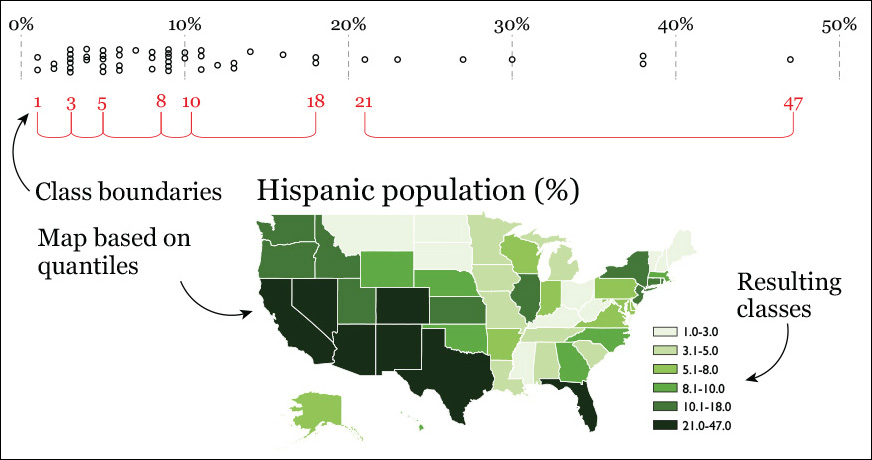
Figure 10.26 Choropleth map based on classes that contain roughly similar number of observations, between seven and ten each.
Also, pay attention to the last class. It’s 21.0 to 47.0, but the upper boundary of the class that precedes it is 18.0. There’s a gap between 18.1 and 21.0 in our color scale because there are no observations in that region of the distribution. Gaps may puzzle readers, so it’s advisable to add a little footnote explaining why they exist.
A third classification method is based on the mean and the standard deviation. This can be helpful to design diverging color schemes, as on Figure 10.27, which is the map that I like the best so far.
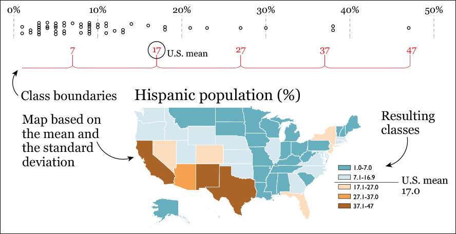
We know that 17 percent of people in the U.S. are Hispanic. That’s our mean. The standard deviation of our data set is close to 10.0. We can use that as our class size. To calculate the class ranges, we begin with the mean, and we add and subtract the standard deviation as many times as needed to include the entire data set, like this:
Below the mean:
Class 1: 17.0 – 10.0 = 7.0
Class 2: 17.0 – (2 × 10.0) = -3.0
There aren’t negative values in our data set, so let’s use the smallest figure (1.0) as the lowest boundary of this class.
Above the mean:
Class 3: 17.0 + 10.0 = 27.0
Class 4: 17.0 + (2 × 10.0) = 37.0
Class 5: 17.0 + (3 × 10.0) = 47.0
In our data set there isn’t any state that matches the national mean of 17 percent. If that were the case, we could consider building a class just for it and use a neutral hue (perhaps light gray) to identify it.
There are many other ways of calculating class size available in GIS (Geographic Information System) and mapping software. A group of methods called optimal tries to find natural breaks between the intervals. One of the most popular among cartographers is the Fisher-Jenks algorithm, which is applied on Figure 10.28. The results are similar to Figure 10.25.

Software tools will also let you design non-classed choropleth maps, in which the color scale is a gradient, as on Figure 10.29.

Using Choropleth Maps
A single choropleth map can be effective at revealing potential stories, but often the best approach when exploring data is to put several maps side by side. Compare Figure 10.30 to Figure 10.31 and Figure 10.32, and see if you notice promising patterns that are worth analyzing with the help of experts in public health statistics.
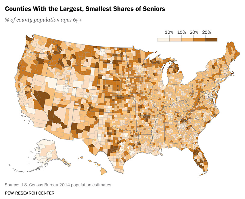
Figure 10.30 Map by the Pew Research Center. Notice the high proportion of seniors in areas like South and West Florida.
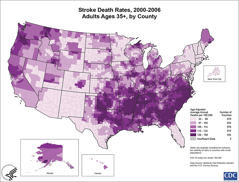
Figure 10.31 Map by Schieb L. “Stroke Death Rates, 2000-2006, Adults Ages 35+, by County.” May 2011. Centers for Disease Control and Prevention. Notice that strokes are more common in the South, but not necessarily in the areas with a higher proportion of elderly people.
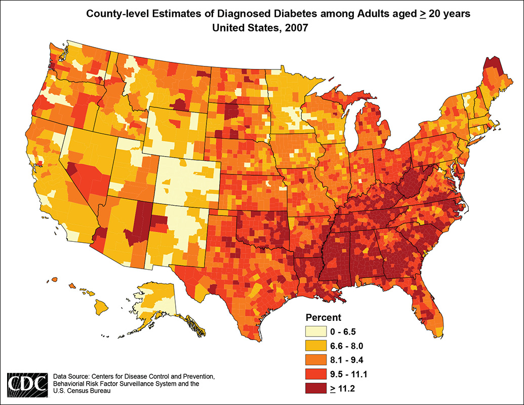
Figure 10.32 Map by Karen Kirtland. 2007 Estimates of the Percentage of Adults with Diagnosed Diabetes Division of Diabetes Translation, Centers for Disease Control and Prevention. Diabetes tends to concentrate in the same counties as stroke.
Maps should often be combined with linked charts or tables to achieve a richer understanding. Figure 10.33 is an interactive visualization by the Berliner Morgenpost that includes a non-classed choropleth map of crime rates per 1,000 people in Berlin, a search box, and a sortable ranking and bar chart.

Figure 10.33 Crime in Berlin. Berliner Morgenpost: http://tinyurl.com/owuf6w6.
The Berliner Morgenpost has published many other fine data maps with elegant color schemes. Figure 10.34 uses shades of blue and orange to identify neighborhoods in the city inhabited mainly by native Berliners or by people born in other places.
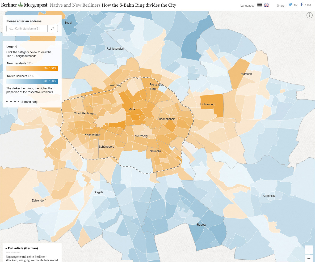
Figure 10.34 “Native and New Berliners.” Berliner Morgenpost: http://tinyurl.com/p8upc94.
The same colors are applied on the diverging color scheme on Figure 10.35: shades of blue for regions in Europe where population shrank between 2001 and 2011, and shades of orange for those that experienced growth. Gray identifies areas that remained unchanged.
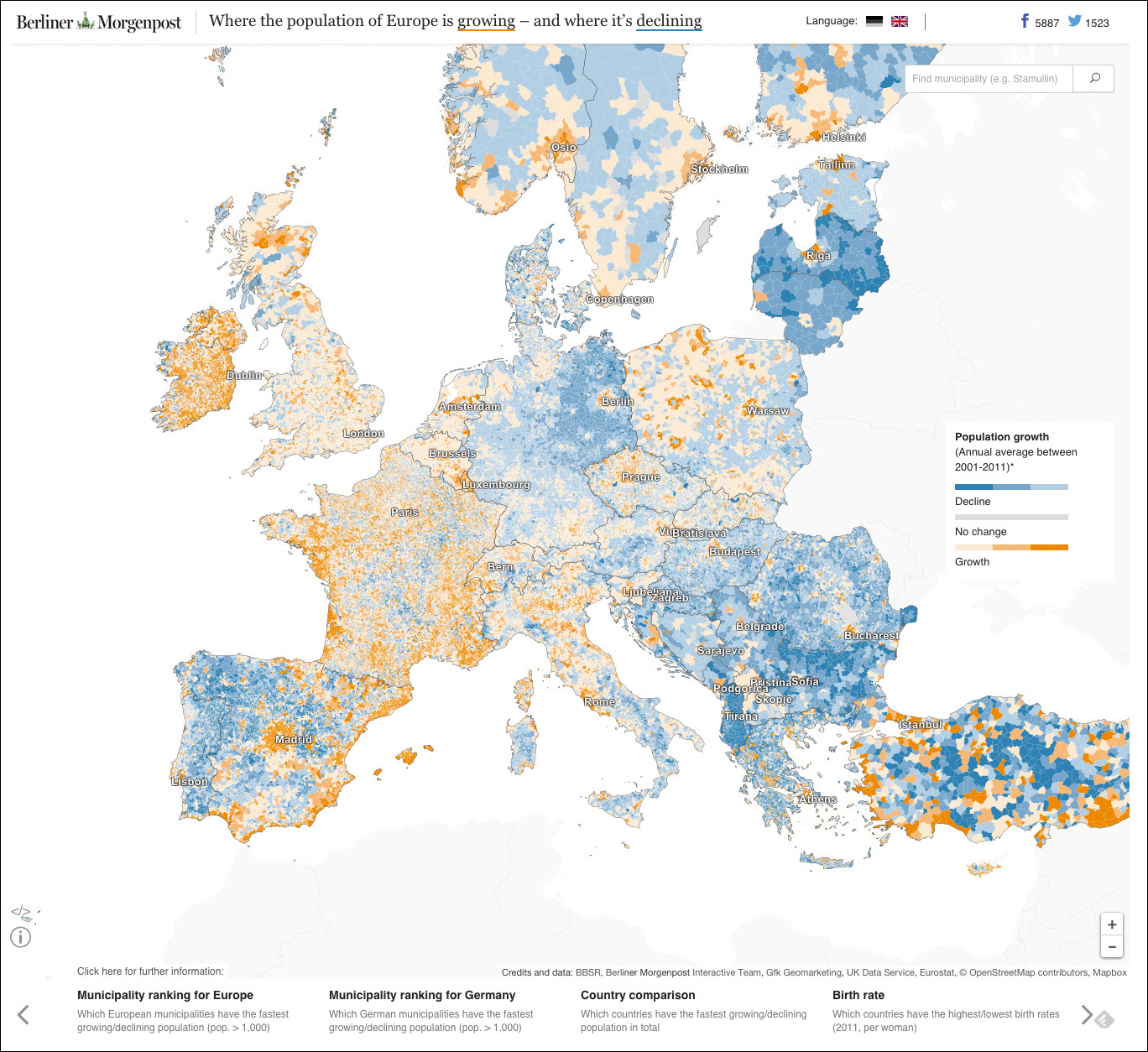
Figure 10.35 “Where the population of Europe is growing—and where it’s declining.” Berliner Morgenpost: http://tinyurl.com/nvq9b49.
Color schemes in choropleth maps can become quite complex. See Figure 10.36 for an example. Here, analysts at the Centers for Disease Control and Prevention (CDC) categorized counties according to poverty rates and spatial concentration. The way classes on this map were calculated isn’t disclosed, unfortunately, but the result is still persuasive.

Figure 10.36 Spatial Concentrations and Outliers of Poverty, United States, 1999 James B. Holt, Centers for Disease Control and Prevention.
A very well-known shortcoming of choropleth maps is that regions in the world vary wildly in size. Imagine that you do a world map of child mortality rates. Large countries such as Brazil, Russia, and the U.S. will stand out, while small countries with relatively large population densities (Israel, Switzerland) will be almost invisible. We face this same problem when designing maps of most countries. In the case of the U.S., large but sparsely populated states like Montana and the Dakotas will look more prominent than small but densely populated ones, like Massachusetts.
There are several strategies to overcome this challenge; most of them are based on disposing of geographical reality and designing very abstract diagrams like the one on Figure 10.37, by ProPublica, where all states are transformed into circles of identical size.
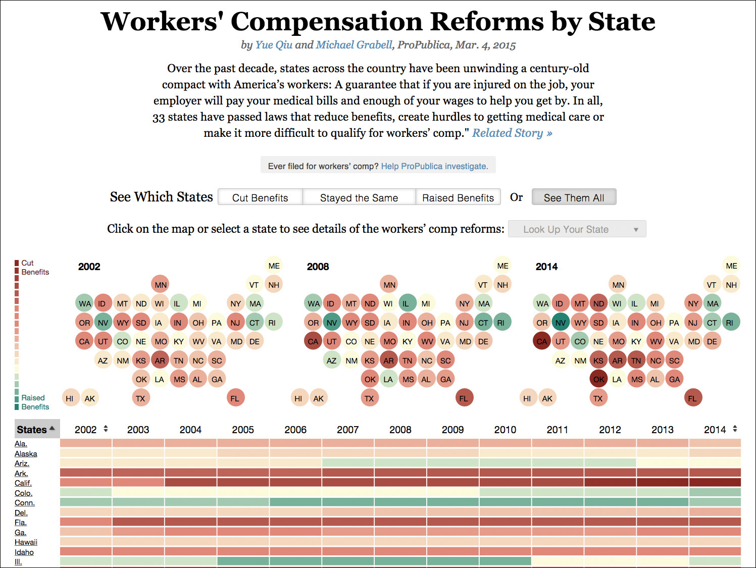
Figure 10.37 “Workers’ Compensation Reforms by State.” ProPublica: http://projects.propublica.org/graphics/workers-comp-reform-by-state.
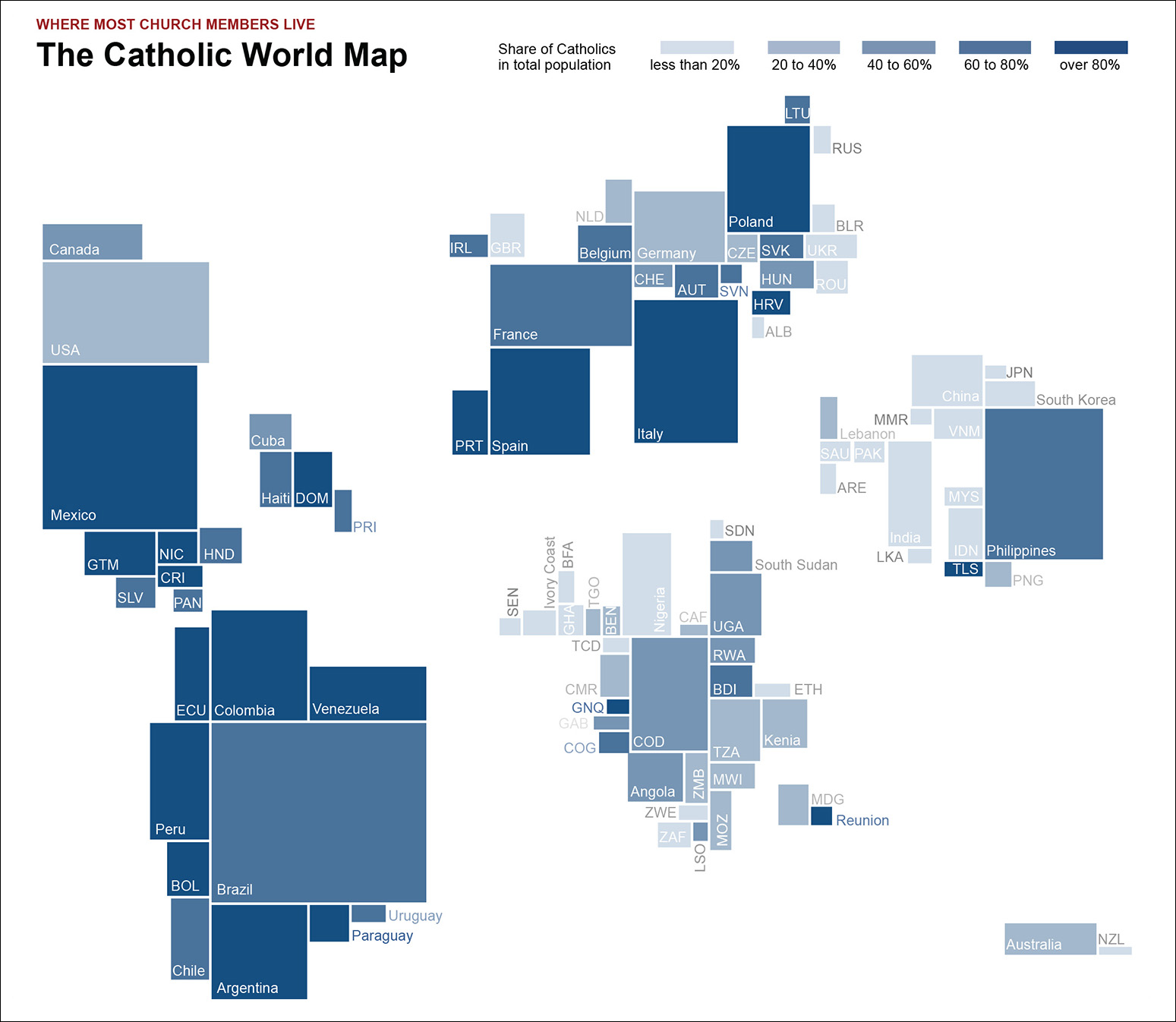
If circles on that visualization had been sized in proportion to population, we’d end up with a cartogram. A cartogram is a map in which areas are scaled up or down based on some magnitude. Figure 10.38, by Zeit Online, is both a cartogram and a choropleth map: each country is represented by a rectangle that expands or shrinks according to the total amount of Catholics. Shades of blue encode the percentage of the population that is Catholic.
Other Kinds of Data Maps
This chapter has covered the basics of proportional symbol maps and choropleth maps, but there are many other kinds of maps capable of displaying data.
Often, data can’t be properly encased within neatly defined spatial units such as countries, provinces, or zip codes. Think of the weather and temperature maps you often see in the news. They are examples of isarithmic maps, or contour maps. Figure 10.39 is a good example. Here, the boundaries of each color splotch are drawn by connecting points of equal value.6 In this case, these points share the same density of deaths due to heart disease.
6 The prefix “iso” means “same,” as in “isomorphism,” which means “having the same form.”

Figure 10.39 Map by Brondum J. “Heart Disease Deaths Kernel Density, Hennepin County, Minnesota.” November 2012. Hennepin County Human Services and Public Health Department.
Shapes in isarithmic maps don’t need to be curvy and smooth. The maps on Figure 10.40 are divided into hexagons that don’t really correspond to any German administrative units.

Figure 10.40 Maps from “A Nation Divided,” Zeit Online: http://zeit.de/feature/german-unification-a-nation-divided. Notice the stark differences between West Germany and East Germany.
Cartographers, designers, and coders are constantly experimenting with unusual map varieties. To end this chapter, I’d like to point out Figure 10.41, an interactive map by Estado de São Paulo. Colors correspond to the party that won in each district in the 2010 Presidential election. Red is PT (Partido dos Trabalhadores) and blue is for PSDB (Partido da Social Democracia Brasileira.)
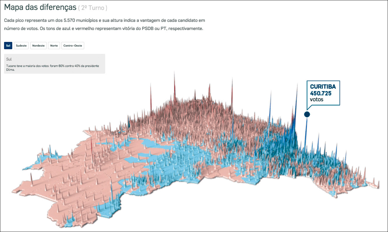
Figure 10.41 Estado de São Paulo. Presidential election results: http://infograficos.estadao.com.br/politica/resultado-eleicoes-2014/.
The height of each peak is proportional to the difference of votes in favor of the winning party. I am not a huge fan of 3D data displays, but this case is special, as readers can rotate the map at will to see it from different angles.
Figure 10.42, by Mike Bostock, and Figure 10.43, by Jason Davies, are Voronoi maps of distances to airports. In Voronoi maps and diagrams, surfaces are tesselated into polygons, each with a dot inside. Each polygon is drawn in a way that all points within it are closer to the central dot than to any other dot on the display. Interact with these maps. You’ll be bewitched.
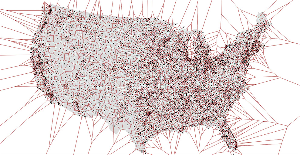
Figure 10.42 Voronoi map of U.S. airports, by Mike Bostock: http://bl.ocks.org/mbostock/4360892.
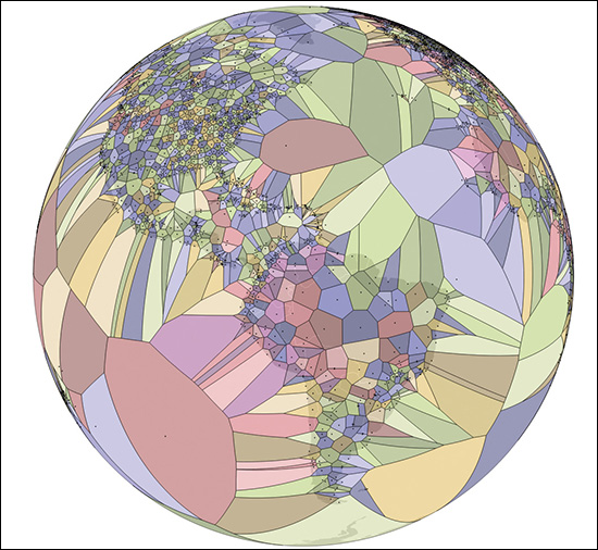
Figure 10.43 Interactive 3D Voronoi map of world airports, by Jason Davies: https://www.jasondavies.com/maps/voronoi/airports/.
To Learn More
• For a good introduction of how to design good color schemes for maps, read Rob Simmon’s series of six articles titled “Subtleties of Color.” You can find them here: http://earthobservatory.nasa.gov/blogs/elegantfigures/2013/08/05/subtleties-of-color-part-1-of-6/.
• ColorBrewer is an excellent follow-up to Simmon’s articles. It lets you choose color schemes that are appropriate for colorblind people and are print-friendly, photocopy-safe, etc. See http://colorbrewer2.org/.
• Brewer, Cynthia. Designing Better Maps: A Guide for GIS Users. Redlands, CA: ESRI, 2005. Brewer is one of the people behind ColorBrewer. This book is an excellent introduction to the principles behind that tool.
• MacEachren, Alan M. How Maps Work: Representation, Visualization, and Design. New York: Guilford, 1995. Its title says it all.
• Monmonier, Mark S. How to Lie with Maps. Chicago: University of Chicago, 1991. This is the most concise primer on map design I’ve ever read. Its title should actually be “How NOT to Lie with Maps.”
• Peterson, Gretchen N. Cartographer’s Toolkit: Colors, Typography, Patterns. Fort Collins, CO: PetersonGIS, 2012. A good book to have by your side when choosing styles for your maps.
• Slocum, Terry A. Thematic Cartography and Geovisualization (3rd edition). Upper Saddle River, NJ: Pearson Prentice Hall, 2009. The bible of data mapping.