Chapter 3. Data all around us: the virtual wilderness
This chapter covers
- Discovering data you may need
- Interacting with data in various environments
- Combining disparate data sets
This chapter discusses the principal species of study of the data scientist: data. Having possession of data—namely, useful data—is often taken as a foregone conclusion, but it’s not usually a good idea to assume anything of the sort. As with any topic worthy of scientific examination, data can be hard to find and capture and is rarely completely understood. Any mistaken notion about a data set that you possess or would like to possess can lead to costly problems, so in this chapter, I discuss the treatment of data as an object of scientific study.
3.1. Data as the object of study
In recent years, there has been a seemingly never-ending discussion about whether the field of data science is merely a reincarnation or an offshoot—in the Big Data Age—of any of a number of older fields that combine software engineering and data analysis: operations research, decision sciences, analytics, data mining, mathematical modeling, or applied statistics, for example. As with any trendy term or topic, the discussion over its definition and concept will cease only when the popularity of the term dies down. I don’t think I can define data science any better than many of those who have done so before me, so let a definition from Wikipedia (https://en.wikipedia.org/wiki/Data_science), paraphrased, suffice:
Data science is the extraction of knowledge from data.
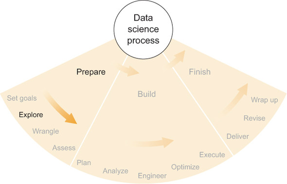
Simple enough, but that description doesn’t distinguish data science from the many other similar terms, except perhaps to claim that data science is an umbrella term for the whole lot. On the other hand, this era of data science has a property that no previous era had, and it is, to me, a fairly compelling reason to apply a new term to the types of things that data scientists do that previous applied statisticians and data-oriented software engineers did not. This reason helps me underscore an often-overlooked but very important aspect of data science, as shown in figure 3.1.
Figure 3.1. The second step of the preparation phase of the data science process: exploring available data
3.1.1. The users of computers and the internet became data generators
Throughout recent history, computers have made incredible advances in computational power, storage, and general capacity to accomplish previously unheard-of tasks. Every generation since the invention of the modern computer nearly a century ago has seen ever-shrinking machines that are orders of magnitude more powerful than the most powerful supercomputers of the previous generation.
The time period including the second half of the twentieth century through the beginning of the twenty-first, and including the present day, is often referred to as the Information Age. The Information Age, characterized by the rise to ubiquity of computers and then the internet, can be divided into several smaller shifts that relate to analysis of data.
First, early computers were used mainly to make calculations that previously took an unreasonable amount of time. Cracking military codes, navigating ships, and performing simulations in applied physics were among the computationally intensive tasks that were performed by early computers.
Second, people began using computers to communicate, and the internet developed in size and capacity. It became possible for data and results to be sent easily across a large distance. This enabled a data analyst to amass larger and more varied data sets in one place for study. Internet access for the average person in a developed country increased dramatically in the 1990s, giving hundreds of millions of people access to published information and data.
Third, whereas early use of the internet by the populace consisted mainly of consuming published content and communication with other people, soon the owners of many websites and applications realized that the aggregation of actions of their users provided valuable insight into the success of their own product and sometimes human behavior in general. These sites began to collect user data in the form of clicks, typed text, site visits, and any other actions a user might take. Users began to produce more data than they consumed.
Fourth, the advent of mobile devices and smartphones that are connected to the internet made possible an enormous advance in the amount and specificity of user data being collected. At any given moment, your mobile device is capable of recording and transmitting every bit of information that its sensors can collect (location, movement, camera image and video, sound, and so on) as well as every action that you take deliberately while using the device. This can potentially be a huge amount of information, if you enable or allow its collection.
Fifth—though this isn’t necessarily subsequent to the advent of personal mobile devices—is the inclusion of data collection and internet connectivity in almost everything electronic. Often referred to as the Internet of Things (IoT), these can include everything from your car to your wristwatch to the weather sensor on top of your office building. Certainly, collecting and transmitting information from devices began well before the twenty-first century, but its ubiquity is relatively new, as is the availability of the resultant data on the internet in various forms, processed or raw, for free or for sale.
Through these stages of growth of computing devices and the internet, the online world became not merely a place for consuming information but a data-collection tool in and of itself. A friend of mine in high school in the late 1990s set up a website offering electronic greeting cards as a front for collecting email addresses. He sold the resulting list of millions of email addresses for a few hundred thousand dollars. This is a primitive example of the value of user data for purposes completely unrelated to the website itself and a perfect example of something I’m sorry to have missed out on in my youth. By the early 2000s, similar-sized collections of email addresses were no longer worth nearly this much money, but other sorts of user data became highly desirable and could likewise fetch high prices.
3.1.2. Data for its own sake
As people and businesses realized that user data could be sold for considerable sums of money, they began to collect it indiscriminately. Very large quantities of data began to pile up in data stores everywhere. Online retailers began to store not only everything you bought but also every item you viewed and every link you clicked. Video games stored every step your avatar ever took and which opponents it vanquished. Various social networks stored everything you and your friends ever did.
The purpose of collecting all of this data wasn’t always to sell it, though that happens frequently. Because virtually every major website and application uses its own data to optimize the experience and effectiveness of users, site and app publishers are typically torn between the value of the data as something that can be sold and the value of the data when held and used internally. Many publishers are afraid to sell their data because that opens up the possibility that someone else will figure out something lucrative to do with it. Many of them keep their data to themselves, hoarding it for the future, when they supposedly will have enough time to wring all value out of it.
Internet juggernauts Facebook and Amazon collect vast amounts of data every minute of every day, but in my estimation, the data they possess is largely unexploited. Facebook is focused on marketing and advertising revenue, when they have one of the largest data sets comprising human behavior all around the world. Product designers, marketers, social engineers, and sociologists alike could probably make great advances in their fields, both academic and industrial, if they had access to Facebook’s data. Amazon, in turn, has data that could probably upend many beloved economic principles and create several new ones if it were turned over to academic institutions. Or it might be able to change the way retail, manufacturing, and logistics work throughout the entire industry.
These internet behemoths know that their data is valuable, and they’re confident that no one else possesses similar data sets of anywhere near the same size or quality. Innumerable companies would gladly pay top dollar for access to the data, but Facebook and Amazon have—I surmise—aspirations of their own to use their data to its fullest extent and therefore don’t want anyone else to grab the resulting profits. If these companies had unlimited resources, surely they would try to wring every dollar out of every byte of data. But no matter how large and powerful they are, they’re still limited in resources, and they’re forced to focus on the uses of the data that affect their bottom lines most directly, to the exclusion of some otherwise valuable efforts.
On the other hand, some companies have elected to provide access to their data. Twitter is a notable example. For a fee, you can access the full stream of data on the Twitter platform and use it in your own project. An entire industry has developed around brokering the sale of data, for profit. A prominent example of this is the market of data from various major stock exchanges, which has long been available for purchase.
Academic and nonprofit organizations often make data sets available publicly and for free, but there may be limitations on how you can use them. Because of the disparity of data sets even within a single scientific field, there has been a trend toward consolidation of both location and format of data sets. Several major fields have created organizations whose sole purpose is to maintain databases containing as many data sets as possible from that field. It’s often a requirement that authors of scientific articles submit their data to one of these canonical data repositories prior to publication of their work.
In whichever form, data is now ubiquitous, and rather than being merely a tool that analysts might use to draw conclusions, it has become a purpose of its own. Companies now seem to collect data as an end, not a means, though many of them claim to be planning to use the data in the future. Independent of other defining characteristics of the Information Age, data has gained its own role, its own organizations, and its own value.
3.1.3. Data scientist as explorer
In the twenty-first century, data is being collected at unprecedented rates, and in many cases it’s not being collected for a specific purpose. Whether private, public, for free, for sale, structured, unstructured, big, normal size, social, scientific, passive, active, or any other type, data sets are accumulating everywhere. Whereas for centuries data analysts collected their own data or were given a data set to work on, for the first time in history many people across many industries are collecting data first and then asking, “What can I do with this?” Still others are asking, “Does the data already exist that can solve my problem?”
In this way data—all data everywhere, as a hypothetical aggregation—has become an entity worthy of study and exploration. In years past, data sets were usually collected deliberately, so that they represented some intentional measurement of the real world. But more recently the internet, ubiquitous electronic devices, and a latent fear of missing out on hidden value in data have led us to collect as much data as possible, often on the loose premise that we might use it later.
Figure 3.2 shows an interpretation of four major innovation types in computing history: computing power itself, networking and communication between computers, collection and use of big data, and rigorous statistical analysis of that big data. By big data, I mean merely the recent movement to capture, organize, and use any and all data possible. Each of these computing innovations begins with a problem that begs to be addressed and then goes through four phases of development, in a process that’s similar to the technological surge cycle of Carlota Perez (Technological Revolutions and Financial Capital, Edward Elgar Publishing, 2002) but with a focus on computing innovation and its effect on computer users and the general public.
Figure 3.2. We’re currently in the refinement phase of big data collection and use and in the widespread adoption phase of statistical analysis of big data.

For each innovation included in the figure, there are five stages:
- Problem— There is a problem that computers can address in some way.
- Invention— The computing technology that can address that problem is created.
- Proof/recognition— Someone uses the computing technology in a meaningful way, and its value is proven or at least recognized by some experts.
- Adoption— The newly proven technology is widely put to use in industry.
- Refinement— People develop new versions, more capabilities, higher efficiency, integrations with other tools, and so on.
Because we’re currently in the refinement phase of big data collection and the widespread adoption phase of statistical analysis of that data, we’ve created an entire data ecosystem wherein the knowledge that has been extracted is only a very small portion of the total knowledge contained. Not only has much of the knowledge not been extracted yet, but in many cases the full extent and properties of the data set are not understood by anyone except maybe a few software engineers who set up the system; the only people who might understand what’s contained in the data are people who are probably too busy or specialized to make use of it. The aggregation of all of this underutilized or poorly understood data to me is like an entirely new continent with many undiscovered species of plants and animals, some entirely unfamiliar organisms, and possibly a few legacy structures left by civilizations long departed.
There are exceptions to this characterization. Google, Amazon, Facebook, and Twitter are good examples of companies that are ahead of the curve. They are, in some cases, engaging in behavior that matches a later stage of innovation. For example, by allowing access to its entire data set (often for a fee), Twitter seems to be operating within the refinement stage of big data collection and use. People everywhere are trying to squeeze every last bit of knowledge out of users’ tweets. Likewise, Google seems to be doing a good job of analyzing its data in a rigorous statistical manner. Its work on search-by-image, Google Analytics, and even its basic text search are good examples of solid statistics on a large scale. One can easily argue that Google has a long way to go, however. If today’s ecosystem of data is like a largely unexplored continent, then the data scientist is its explorer. Much like famous early European explorers of the Americas or Pacific islands, a good explorer is good at several things:
- Accessing interesting areas
- Recognizing new and interesting things
- Recognizing the signs that something interesting might be close
- Handling things that are new, unfamiliar, or sensitive
- Evaluating new and unfamiliar things
- Drawing connections between familiar things and unfamiliar things
- Avoiding pitfalls
An explorer of a jungle in South America may have used a machete to chop through the jungle brush, stumbled across a few loose-cut stones, deduced that a millennium-old temple was nearby, found the temple, and then learned from the ruins about the religious rituals of the ancient tribe. A data scientist might hack together a script that pulls some social networking data from a public API, realize that a few people compose major hubs of social activity, discover that those people often mention a new photo-sharing app in their posts on the social network, pull more data from the photo-sharing app’s public API, and in combining the two data sets with some statistical analysis learn about the behavior of network influencers in online communities. Both cases derive previously unknown information about how a society operates. Like an explorer, a modern data scientist typically must survey the landscape, take careful note of surroundings, wander around a bit, and dive into some unfamiliar territory to see what happens. When they find something interesting, they must examine it, figure out what it can do, learn from it, and be able to apply that knowledge in the future. Although analyzing data isn’t a new field, the existence of data everywhere—often regardless of whether anyone is making use of it—enables us to apply the scientific method to discovery and analysis of a preexisting world of data. This, to me, is the differentiator between data science and all of its predecessors. There’s so much data that no one can possibly understand it all, so we treat it as a world unto itself, worthy of exploration.
This idea of data as a wilderness is one of the most compelling reasons for using the term data science instead of any of its counterparts. To get real truth and useful answers from data, we must use the scientific method, or in our case, the data scientific method:
- Ask a question.
- State a hypothesis about the answer to the question.
- Make a testable prediction that would provide evidence in favor of the hypothesis if correct.
- Test the prediction via an experiment involving data.
- Draw the appropriate conclusions through analyses of experimental results.
In this way, data scientists are merely doing what scientists have been doing for centuries, albeit in a digital world. Today, some of our greatest explorers spend their time in virtual worlds, and we can gain powerful knowledge without ever leaving our computers.
3.2. Where data might live, and how to interact with it
Before we dive in to the unexplored wilderness that is the state of data today, I’d like to discuss the forms that data might take, what those forms mean, and how we might treat them initially. Flat files, XML, and JSON are a few data formats, and each has its own properties and idiosyncrasies. Some are simpler than others or more suited to certain purposes. In this section, I discuss several types of formats and storage methods, some of their strengths and weaknesses, and how you might take advantage of them.
Although plenty of people will object to this, I decided to include in this section a discussion of databases and APIs as well. Commingling a discussion of file formats with software tools for data storage makes sense to me because at the beginning of a data science project, any of these formats or data sources is a valid answer to the question “Where is the data now?” File, database, or API, what the data scientist needs to know is “How do I access and extract the data I need?” and so that’s my purpose here.
Figure 3.3 shows three basic ways a data scientist might access data. It could be a file on a file system, and the data scientist could read the file into their favorite analysis tool. Or the data could be in a database, which is also on a file system, but in order to access the data, the data scientist has to use the database’s interface, which is a software layer that helps store and extract data. Finally, the data could be behind an application programming interface (API), which is a software layer between the data scientist and some system that might be completely unknown or foreign. In all three cases, the data can be stored and/or delivered to the data scientist in any format I discuss in this section or any other. Storage and delivery of data are so closely intertwined in some systems that I choose to treat them as a single concept: getting data into your analysis tools.
Figure 3.3. Three ways a data scientist might access data: from a file system, database, or API

In no way do I purport to cover all possible data formats or systems, nor will I list all technical details. My goal here is principally to give descriptions that would make a reader feel comfortable talking about and approaching each one. I can still remember when extracting data from a conventional database was daunting for me, and with this section I’d like to put even beginners at ease. Only if you’re fairly comfortable with these basic forms of data storage and access can you move along to the most important part of data science: what the data can tell you.
3.2.1. Flat files
Flat files are plain-vanilla data sets, the default data format in most cases if no one has gone through the effort to implement something else. Flat files are self-contained, and you don’t need any special programs to view the data contained inside. You can open a flat file for viewing in a program typically called a text editor, and many text editors are available for every major operating system. Flat files contain ASCII (or UTF-8) text, each character of text using (most likely) 8 bits (1 byte) of memory/storage. A file containing only the word DATA will be of size 32 bits. If there is an end-of-line (EOL) character after the word DATA, the file will be 40 bits, because an EOL character is needed to signify that a line has ended. My explanation of this might seem simplistic to many people, but even some of these basic concepts will become important later on as we discuss other formats, so I feel it’s best to outline some basic properties of the flat file so that we might compare other data formats later.
There are two main subtypes of the flat file: plain text and delimited. Plain text is words, as you might type them on your keyboard. It could look like this:
This is what a plain text flat file looks like. It's just plain ASCII text. Lines don't really end unless there is an end-of-line character, but some text editors will wrap text around anyway, for convenience.
Usually, every character is a byte, and so there are only 256 possible characters, but there are a lot of caveats to that statement, so if you're really interested, consult a reference about ASCII and UTF-8.
This file would contain seven lines, or technically eight if there’s an end-of-line character at the end of the final line of text. A plain text flat file is a bunch of characters stored in one of two (or so) possible very common formats. This is not the same as a text document stored in a word processor format, such as Microsoft Word or Open-Office Writer. (See the subsection “Common bad formats.”) Word processor file formats potentially contain much more information, including overhead such as style formats and metadata about the file format itself, as well as objects like images and tables that may have been inserted into a document. Plain text is the minimal file format for containing words and only words—no style, no fancy images. Numbers and some special characters are OK too.
But if your data contains numerous entries, a delimited file might be a better idea. A delimited file is plain text but with the stipulation that every so often in the file a delimiter will appear, and if you line up the delimiters properly, you can make something that looks like a table, with rows, columns, and headers. A delimited file might look like this:
NAME      ID   COLOR     DONE
Alison    1    'blue'    FALSE
Brian     2    'red'     TRUE
Clara     3    'brown'   TRUE
Let’s call this table JOBS_2015, because it represents a fictional set of house-painting jobs that started in 2015, with the customer name, ID, paint color, and completion status.
This table happens to be tab-delimited—or tab-separated value (TSV)—meaning that columns are separated by the tab character. If opened in a text editor, such a file would usually appear as it does here, but it might optionally display the text where a tab would otherwise appear. This is because a tab, like an end-of-line character, can be represented with a single ASCII character, and that character is typically represented with , if not rendered as variable-length whitespace that aligns characters into a tabular format.
If JOBS_2015 were stored as a comma-separated value (CSV) format, it would appear like this in a standard text editor:
NAME,ID,COLOR,DONE
Alison,1,'blue',FALSE
Brian,2,'red',TRUE
Clara,3,'brown',TRUE
The commas have taken the place of the tab characters, but the data is still the same. In either case, you can see that the data in the file can be interpreted as a set of rows and columns. The rows represent one job each for Alison, Brian, and Clara, and the column names on the header (first) line are NAME, ID, COLOR, and DONE, giving the types of details of the job contained within the table.
Most programs, including spreadsheets and some programming languages, require the same number of delimiters on each line (except possibly the header line) so that when they try to read the file, the number of columns is consistent, and each line contributes exactly one entry to each column. Some software tools don’t require this, and they each have specific ways of dealing with varying numbers of entries on each line.
I should note here that delimited files are typically interpreted as tables, like spreadsheets. Furthermore, as plain text files can be read and stored using a word processing program, delimited files can typically be loaded into a spreadsheet program like Microsoft Excel or OpenOffice Calc.
Any common program for manipulating text or tables can read flat files. Popular programming languages all include functions and methods that can read such files. My two most familiar languages, Python (the csv package) and R (the read.table function and its variants), contain methods that can easily load a CSV or TSV file into the most relevant data types in those languages. For plain text also, Python (readlines) and R (readLines) have methods that read a file line by line and allow for the parsing of the text via whatever methods you see fit. Packages in both languages—and many others—provide even more functionality for loading files of related types, and I suggest looking at recent language and package documentation to find out whether another file-loading method better suits your needs.
Without compressing files, flat files are more or less the smallest and simplest common file formats for text or tables. Other file formats contain other information about the specifics of the file format or the data structure, as appropriate. Because they’re the simplest file formats, they’re usually the easiest to read. But because they’re so lean, they provide no additional functionality other than showing the data, so for larger data sets, flat files become inefficient. It can take minutes or hours for a language like Python to scan a flat file containing millions of lines of text. In cases where reading flat files is too slow, there are alternative data storage systems designed to parse through large amounts of data quickly. These are called databases and are covered in a later section.
3.2.2. HTML
A markup language is plain text marked up with tags or specially denoted instructions for how the text should be interpreted. The very popular Hypertext Markup Language (HTML) is used widely on the internet, and a snippet might look like this:
<html>
    <body>
        <div class="column">
            <h1>Column One</h1>
            <p>This is a paragraph</p>
        </div>

        <div class="column">
            <h1>Column Two</h1>
            <p>This is another paragraph</p>
        </div>
    </body>
</html>
An HTML interpreter knows that everything between the <html> and </html> tags should be considered and read like HTML. Similarly, everything between the <body> and </body> tags will be considered the body of the document, which has special meaning in HTML rendering. Most HTML tags are of the format <TAGNAME> to begin the annotation and </TAGNAME> to end it, for an arbitrary TAGNAME. Everything between the two tags is now treated as being annotated by TAGNAME, which an interpreter can use to render the document. The two <div> tags in the example show how two blocks of text and other content can be denoted, and a class called column is applied to the div, allowing the interpreter to treat a column instance in a special way.
HTML is used primarily to create web pages, and so it usually looks more like a document than a data set, with a header, body, and some style and formatting information. HTML is not typically used to store raw data, but it’s certainly capable of doing so. In fact, the concept of web scraping usually entails writing code that can fetch and read web pages, interpreting the HTML, and scraping out the specific pieces of the HTML page that are of interest to the scraper.
For instance, suppose we’re interested in collecting as many blog posts as possible and that a particular blogging platform uses the <div class="column"> tag to denote columns in blog posts. We could write a script that systematically visits a blog, interprets the HTML, looks for the <div class="column"> tag, captures all text between it and the corresponding </div> tag, and discards everything else, before proceeding to another blog to do the same. This is web scraping, and it might come in handy if the data you need isn’t contained in one of the other more friendly formats. Web scraping is sometimes prohibited by website owners, so it’s best to be careful and check the copyright and terms of service of the site before scraping.
3.2.3. XML
Extensible Markup Language (XML) can look a lot like HTML but is generally more suitable for storing and transmitting documents and data other than web pages. The previous snippet of HTML can be valid XML, though most XML documents begin with a tag that declares a particular XML version, such as the following:
<?xml version="1.0" encoding="UTF-8"?>
This declaration helps ensure that an XML interpreter reads tags in the appropriate way. Otherwise, XML works similarly to HTML but without most of the overhead associated with web pages. XML is now used as a standard format for offline documents such as the OpenOffice and Microsoft Office formats. Because the XML specification is designed to be machine-readable, it also can be used for data transmission, such as through APIs. For example, many official financial documents are available publicly in the Extensible Business Reporting Language (XBRL), which is XML-based.
This is a representation of the first two rows of the table JOBS_2015 in XML:
<JOB>
     <NAME>Alison</NAME>
     <ID>1</ID>
     <COLOR>'blue'</COLOR>
     <DONE>FALSE</DONE>
</JOB>
<JOB>
     <NAME>Brian</NAME>
     <ID>2</ID>
     <COLOR>'red'</COLOR>
     <DONE>TRUE</DONE>
</JOB>
You can see that each row of the table is denoted by a <JOB> tag, and within each JOB, the table’s column names have been used as tags to denote the various fields of information. Clearly, storing data in this format takes up more disk space than a standard table because XML tags take up disk space, but XML is much more flexible, because it’s not limited to a row-and-column format. For this reason, it has become popular in applications and documents using non-tabular data and other formats requiring such flexibility.
3.2.4. JSON
Though not a markup language, JavaScript Object Notation (JSON) is functionally similar, at least when storing or transmitting data. Instead of describing a document, JSON typically describes something more like a data structure, such as a list, map, or dictionary in many popular programming languages. Here’s the data from the first two rows of the table JOBS_2015 in JSON:
[
     {
          NAME: "Alison",
          ID: 1,
          COLOR: "blue",
          DONE: False
     },
     {
          NAME: "Brian",
          ID: 2,
          COLOR: "red",
          DONE: True
     }
]
In terms of structure, this JSON representation looks a lot like the XML representation you’ve already seen. But the JSON representation is leaner in terms of the number of characters needed to express the data, because JSON was designed to represent data objects and not as a document markup language. Therefore, for transmitting data, JSON has become very popular. One huge benefit of JSON is that it can be read directly as JavaScript code, and many popular programming languages including Python and Java have natural representations of JSON as native data objects. For interoperability between programming languages, JSON is almost unparalleled in its ease of use.
3.2.5. Relational databases
Databases are data storage systems that have been optimized to store and retrieve data as efficiently as possible within various contexts. Theoretically, a relational database (the most common type of database) contains little more than a set of tables that could likewise be represented by a delimited file, as already discussed: row and column names and one data point per row-column pair. But databases are designed to search—or query, in the common jargon—for specific values or ranges of values within the entries of the table.
For example, let’s revisit the JOBS_2015 table:
NAME      ID     COLOR     DONE
Alison    1     'blue'     FALSE
Brian     2     'red'      TRUE
Clara     3     'brown'    TRUE
But this time assume that this table is one of many stored in a database. A database query could be stated in plain English as follows:
From JOBS_2015, show me all NAME in rows where DONE=TRUE
This query should return the following:
Brian
Clara
That’s a basic query, and every database has its own language for expressing queries like this, though many databases share the same basis query language, the most common being Structured Query Language (SQL).
Now imagine that the table contains millions of rows and you’d like to do a query similar to the one just shown. Through some tricks of software engineering, which I won’t discuss here, a well-designed database is able to retrieve a set of table rows matching certain criteria (a query) much faster than a scan of a flat file would. This means that if you’re writing an application that needs to search for specific data very often, you may improve retrieval speed by orders of magnitude if you use a database instead of a flat file.
The main reason why databases are good at retrieving specific data quickly is the database index. A database index is itself a data structure that helps that database software find relevant data quickly. It’s like a structural map of the database content, which has been sorted and stored in a clever way and might need to be updated every time data in the database changes. Database indexes are not universal, however, meaning that the administrator of the database needs to choose which columns of the tables are to be indexed, if the default settings aren’t appropriate. The columns that are chosen to be indexed are the ones upon which querying will be most efficient, and so the choice of index is an important one for the efficiency of your applications that use that database.
Besides querying, another operation that databases are typically good at is joining tables. Querying and joining aren’t the only two things that databases are good at, but they’re by far the most commonly utilized reasons to use a database over another data storage system. Joining, in database jargon, means taking two tables of data and combining them to make another table that contains some of the information of both of the original tables.
For example, assume you have the following table, named CUST_ZIP_CODES:
CUST_ID  ZIP_CODE
1        21230
2        45069
3        21230
4        98033
You’d like to investigate which paint colors have been used in which ZIP codes in 2015. Because the colors used on the various jobs are in JOBS_2015 and the customers’ ZIP codes are in CUST_ZIP_CODES, you need to join the tables in order to match colors with ZIP codes. An inner join matching ID from table JOBS_2015 and CUST_ID from table CUST_ZIP_CODES could be stated in plain English:
JOIN tables JOBS_2015 and CUST_ZIP_CODES where ID equals CUST_ID, and
show me ZIP_CODE and COLOR.
You’re telling the database to first match up the customer ID numbers from the two tables and then show you only the two columns you care about. Note that there are no duplicate column names between the two tables, so there’s no ambiguity in naming. But in practice you’d normally have to use a notation like CUST_ZIP_CODES.CUST_ID to denote the CUST_ID column of CUST_ZIP_CODES. I use the shorter version here for brevity.
The result of the join would look like this:
ZIP_CODE    COLOR
21230       'blue'
45069       'red'
21230       'brown'
Joining can be a very big operation if the original tables are big. If each table had millions of different IDs, it could take a long time to sort them all and match them up. Therefore, if you’re joining tables, you should minimize the size of those tables (primarily by number of rows) because the database software will have to shuffle all rows of both tables based on the join criteria until all appropriate combinations of rows have been created in the new table. Joins should be done sparingly and with care.
It’s a good general rule, if you’re going to query and join, to query the data first before joining. For example, if you care only about the COLOR in ZIP_CODE 21230, it’s usually better to query CUST_ZIP_CODES for ZIP_CODE=21230 first and join the result with JOBS_2015 instead of joining first and then querying. This way, there might be far less matching to do, and the execution of the operation will be much faster overall. For more information and guidance on optimizing database operations, you’ll find plenty of practical database books in circulation.
You can think of databases in general as well-organized libraries, and their indexes are good librarians. A librarian can find the book you need in a matter of seconds, when it might have taken you quite a long time to find it yourself. If you have a relatively large data set and find that your code or software tool is spending a lot of time searching for the data it needs at any given moment, setting up a database is certainly worth considering.
3.2.6. Non-relational databases
Even if you don’t have tabular data, you might still be able to make use of the efficiency of database indexing. An entire genre of databases called NoSQL (often interpreted as “Not only SQL”) allows for database schemas outside the more traditional SQL-style relational databases. Graph databases and document databases are typically classified as NoSQL databases.
Many NoSQL databases return query results in familiar formats. Elasticsearch and MongoDB, for instance, return results in JSON format (discussed in section 3.2.4). Elasticsearch in particular is a document-oriented database that’s very good at indexing the contents of text. If you’re working with numerous blog posts or books, for example, and you’re performing operations such as counting the occurrences of words within each blog post or book, then Elasticsearch is typically a good choice, if indexed properly.
Another possible advantage of some NoSQL databases is that, because of the flexibility of the schema, you can put almost anything into a NoSQL database without much hassle. Strings? Maps? Lists? Sure! Why not? MongoDB, for instance, is extremely easy to set up and use, but then you do lose some performance that you might have gained by setting up a more rigorous index and schema that apply to your data.
All in all, if you’re working with large amounts of non-tabular data, there’s a good chance that someone has developed a database that’s good at indexing, querying, and retrieving your type of data. It’s certainly worth a quick look around the internet to see what others are using in similar cases.
3.2.7. APIs
An application programming interface (API) in its most common forms is a set of rules for communicating with a piece of software. With respect to data, think of an API as a gateway through which you can make requests and then receive the data, using a well-defined set of terms. Databases have APIs; they define the language that you must use in your query, for instance, in order to receive the data you want.
Many websites also have APIs. Tumblr, for instance, has a public API that allows you to ask for and receive information about Tumblr content of certain types, in JSON format. Tumblr has huge databases containing all the billions of posts hosted on its blogging service. But it has decided what you, as a member of the public, can and can’t access within the databases. The methods of access and the limitations are defined by the API.
Tumblr’s API is a REST API accessible via HTTP. I’ve never found the technical definition of REST API to be helpful, but it’s a term that people use when discussing APIs that are accessible via HTTP—meaning you can usually access them from a web browser—and that respond with information in a familiar format. For instance, if you register with Tumblr as a developer (it’s free), you can get an API key. This API key is a string that’s unique to you, and it tells Tumblr that you’re the one using the API whenever you make a request. Then, in your web browser, you can paste the URL http://api.tumblr.com/v2/blog/good.tumblr.com/info?api_key=API_KEY, which will request information about a particular blog on Tumblr (replacing API_KEY with the API key that you were given). After you press Enter, the response should appear in your browser window and look something like this (after some reformatting):
{
    meta:
    {
        status: 200,
        msg: "OK"
    },
    response:
    {
        blog:
        {
            title: "",
            name: "good",
            posts: 2435,
            url: "http://good.tumblr.com/",
            updated: 1425428288,
            description: "<font size="6">
                        GOOD is a magazine for the global citizen.
                        </font>",
            likes: 429
        }
    }
}
This is JSON with some HTML in the description field. It contains some metadata about the status of the request and then a response field containing the data that was requested. Assuming you know how to parse JSON strings (and likewise HTML), you can use this in a programmatic way. If you were curious about the number of likes of Tumblr blogs, you could use this API to request information about any number of blogs and compare the numbers of likes that they have received. You wouldn’t want to do that, though, from your browser window, because it would take a very long time.
In order to capture the Tumblr API response programmatically, you need to use an HTTP or URL package in your favorite programming language. In Python there is urllib, in Java HttpUrlConnection, and R has url, but there are many other packages for each of these languages that perform similar tasks. In any case, you’ll have to assemble the request URL (as a string object/variable) and then pass that request to the appropriate URL retrieval method, which should return a response similar to the previous one that can be captured as another object/variable. Here’s an example in Python:
import urllib

requestURL =
    'http://api.tumblr.com/v2/blog/good.tumblr.com/info?api_key=API_KEY'

response = urllib.urlopen(requestURL)
After running these lines, the variable response should contain a JSON string that looks similar to the response shown.
I remember learning how to use an API like this one from Python, and I was a bit confused and overwhelmed at first. Getting the request URL exactly right can be tricky if you’re assembling it programmatically from various parts (for example, base URL, parameters, API key, and so on). But being adept at using APIs like this one can be one of the most powerful tools in data collection, because so much data is available through these gateways.
3.2.8. Common bad formats
It’s no secret that I’m not a fan of the typical suites of office software: word processing programs, spreadsheets, mail clients. Thankfully, I’m not often required to use them. I avoid them whenever possible and never more so than when doing data science. That doesn’t mean that I won’t deal with those files; on the contrary, I wouldn’t throw away free data. But I make sure to get away from any inconvenient formats as quickly as possible. There usually isn’t a good way to interact with them unless I’m using the highly specialized programs that were built for them, and these programs typically aren’t capable of the analysis that a data scientist usually needs. I can’t remember the last time I did (or saw) a solid bit of data science in Microsoft Excel; to me, Excel’s methods for analysis are limited, and the interface is unwieldy for anything but looking at tables. But I know I’m biased, so don’t mind me if you’re convinced you can do rigorous analysis within a spreadsheet. OpenOffice Calc and Microsoft Excel both allow you to export individual sheets from a spreadsheet into CSV formats. If a Microsoft Word document contains text I’d like to use, I export it either into plain text or maybe HTML or XML.
A PDF can be a tricky thing as well. I’ve exported lots of text (or copied and pasted) from PDFs into plain text files that I then read into a Python program. This is one of my favorite examples of data wrangling, a topic I devote an entire chapter to, and so for now it will suffice to say that exporting or scraping text from a PDF (where possible) is usually a good idea whenever you want to analyze that text.
3.2.9. Unusual formats
This is the umbrella category for all data formats and storage systems with which I’m unfamiliar. All sorts of formats are available, and I’m sure someone had a good reason to develop them, but for whatever reason they’re not familiar to me. Sometimes they’re archaic; maybe they were superseded by another format, but some legacy data sets haven’t yet been updated.
Sometimes the formats are highly specialized. I once participated in a project exploring the chemical structure of a compound and its connection to the way the compound smelled (its aroma). The RDKit package (www.rdkit.org) provided a ton of helpful functionality for parsing through chemical structures and substructures. But much of this functionality was highly specific to chemical structure and its notation. Plus the package made heavy use of a fairly sophisticated binary representation of certain aspects of chemical structure that greatly improved the computational efficiency of the algorithms but also made them extremely difficult to understand.
Here’s what I do when I encounter a data storage system unlike anything I’ve seen before:
- Search and search (and search) online for a few examples of people doing something similar to what I want to do. How difficult might it be to adapt these examples to my needs?
- Decide how badly I want the data. Is it worth the trouble? What are the alternatives?
- If it’s worth it, I try to generalize from the similar examples I found. Sometimes I can gradually expand from examples by fiddling with parameters and methods. I try a few things and see what happens.
Dealing with completely unfamiliar data formats or storage systems can be its own type of exploration, but rest assured that someone somewhere has accessed the data before. If no one has ever accessed the data, then someone was completely mistaken in creating the data format in the first place. When in doubt, send a few emails and try to find someone who can help you.
3.2.10. Deciding which format to use
Sometimes you don’t have a choice. The data comes in a certain format, and you have to deal with it. But if you find that format inefficient, unwieldy, or unpopular, you’re usually free to set up a secondary data store that might make things easier, but at the additional cost of the time and effort it takes you to set up the secondary data store. For applications where access efficiency is critical, the cost can be worth it. For smaller projects, maybe not. You’ll have to cross that bridge when you get there.
I’ll conclude this section with a few general rules about what data formats to use, when you have a choice, and in particular when you’re going to be accessing the data from a programming language. Table 3.1 gives the most common good format for interacting with data of particular types.
Table 3.1. Some common types of data and formats that are good for storing them
|
Type of data |
Good, common format |
|---|---|
| Tabular data, small amount | Delimited flat file |
| Tabular data, large amount with lots of searching/querying | Relational database |
| Plain text, small amount | Flat file |
| Plain text, large amount | Non-relational database with text search capabilities |
| Transmitting data between components | JSON |
| Transmitting documents | XML |
And here are a few guidelines for choosing or converting data formats:
- For spreadsheets and other office documents, export!
- More common formats are usually better for your data type and application.
- Don’t spend too much time converting from a certain format to your favorite; weigh the costs and benefits first.
Now that I’ve covered many of the forms in which data might be presented to you, hopefully you’ll feel somewhat comfortable in a high-level conversation about data formats, stores, and APIs. As always, never hesitate to ask someone for details about a term or system you haven’t heard of before. New systems are being developed constantly, and in my experience, anyone who recently learned about a system is usually eager to help others learn about it.
3.3. Scouting for data
The previous section discussed many of the common forms that data takes, from file formats to databases to APIs. I intended to make these data forms more approachable, as well as to increase awareness about the ways you might look for data. It’s not hard to find data, much like it’s not hard to find a tree or a river (in certain climates). But finding the data that can help you solve your problem is a different story. Or maybe you already have data from an internal system. It may seem like that data can answer the major questions of your project, but you shouldn’t take it for granted. Maybe a data set out there will perfectly complement the data you already have and greatly improve results. There’s so much data on the internet and elsewhere; some part of it should be able to help you. Even if not, a quick search is certainly worth it, even for a long-shot possibility.
In this section, I discuss the act of looking for data that might help you with your project. This is the exploration I talked about at the beginning of this chapter. Now that you have some exposure to common forms of data from the previous section, you can focus less on the format and more on the content and whether it can help you.
3.3.1. First step: Google search
This may seem obvious, but I still feel like mentioning it: Google searches are not perfect. To make them work as well as possible, you have to know what to search for and what you’re looking for in the search results. Given the last section’s introduction to data formats, you now have a little more ammunition for Google searches than before.
A Google search for “Tumblr data” gives different results from a search for “Tumblr API.” I’m not sure which I prefer, given that I don’t have a specific project involving Tumblr at the moment. The former returns results involving the term data as used on Tumblr posts as well as third parties selling historical Tumblr data. The latter returns results that deal almost exclusively with the official Tumblr API, which contains considerable up-to-the-minute information about Tumblr posts. Depending on your project, one might be better than the other.
But it’s definitely worth keeping in mind that terms such as data and API do make a difference in web searches. Try the searches “social networking” and “social networking API.” There’s a dramatic difference in results.
Therefore, when searching for data related to your project, be sure to include modifying terms like historical, API, real time, and so on, because they do make a difference. Likewise, watch out for them in the search results. This may be obvious, but it makes a considerable difference in your ability to find what you’re looking for, and so it’s worth repeating.
3.3.2. Copyright and licensing
I’ve talked about searching for, accessing, and using data, but there’s another very important concern: are you allowed to use it?
As with software licenses, data may have licensing, copyright, or other restrictions that can make it illegal to use the data for certain purposes. If the data comes from academic sources, for example (universities, research institutions, and the like), then there’s often a restriction that the data can’t be used for profit. Proprietary data, such as that of Tumblr or Twitter, often comes with the restriction that you can’t use the data to replicate functionality that the platform itself provides. You may not be able to make a Tumblr client that does the same things as the standard Tumblr platform, but perhaps if you offer other functionality not included in the platform, there would be no restriction. Restrictions like these are tricky, and it’s best to read any legal documentation that the data provider offers. In addition, it’s usually good to search for other examples of people and companies using the data in a similar way and see if there are any references to legal concerns. Precedent is no guarantee that a particular use of the data is legally sound, but it may provide guidance in your decision to use the data or not.
All in all, you should remain keenly aware that most data sets not owned by you or your organization come with restrictions on use. Without confirming that your use case is legal, you remain at risk of losing access to the data or, even worse, a lawsuit.
3.3.3. The data you have: is it enough?
Let’s say you’ve found data and confirmed that you’re allowed to use it for your project. Should you keep looking for more data, or should you attack the data you have immediately? The answer to this question is—like pretty much everything in data science—tricky. In this case, the answer is tricky because data sets aren’t always what they seem to be or what you want them to be. Take the example of Uber, the taxi service app publisher. I recently read that Uber was compelled (upon losing an appeal) to turn over trip data to New York City’s Taxi and Limousine Commission (TLC). Suppose you’re an employee of the TLC, and you’d like to compare Uber with traditional taxi services in regard to the number of trips taken by riders over many specific routes. Given that you have data from both Uber and traditional taxis, it may seem straightforward to compare the number of trips for similar routes between the two types of car services. But once you begin your analysis, you realize that Uber had provided pick-up and drop-off locations in terms of ZIP codes, which happen to be the minimum specificity required by the TLC. ZIP codes can cover large areas, though admittedly less so in New York City than anywhere else. Addresses, or at least city blocks, would have been considerably better from a data analysis perspective, but requiring such specificity presents legal troubles regarding the privacy of personal data of the users of taxi services, so it’s understandable.
So what should you do? After the first waves of disappointment wear off, you should probably check to see whether your data will suffice after all or if you need to supplement this data and/or amend your project plans. There’s often a simple way to accomplish this: can you run through a few specific examples of your intended analyses and see if it makes a significant difference?
In this taxi-versus-Uber example, you’d like to find out whether the relative non-specificity of ZIP code can still provide a useful approximation for the many routes you’d like to evaluate. Pick a specific route, say Times Square (ZIP code: 10036) to the Brooklyn Academy of Music (ZIP code: 11217). If a car travels between 10036 and 11217, what other specific routes might the rider have taken? In this case, those same ZIP codes could also describe a trip from the Intrepid Sea, Air & Space Museum to Grand Army Plaza, or likewise a trip from a restaurant in Hell’s Kitchen to an apartment in Park Slope. These probably don’t mean much to people outside the New York City area, but for our purposes it suffices to say that these other locations are up to a kilometer from the origin and destination of the chosen route, a distance that’s about a ten-minute walk and, by NYC standards, not very short. It’s up to you, the data scientist, to make a decision about whether these other locations in the same ZIP codes are close enough or too far from their intended targets. And this decision, in turn, should be made based on the project’s goals and the precise questions (from chapter 2) that you’re hoping to answer.
3.3.4. Combining data sources
If you find that your data set is insufficient to answer your questions, and you can’t find a data set that is sufficient, it might still be possible to combine data sets to find answers. This is yet another point that seems obvious at times but is worth mentioning because of its importance and because of a few tricky points that might pop up.
Combining two (or more) data sets can be like fitting puzzle pieces together. If the puzzle is, metaphorically, the complete data set you wish you had, then each piece of the puzzle—a data set—needs to cover precisely what the other pieces don’t. Sure, unlike puzzle pieces, data sets can overlap in some sense, but any gap left after all the present pieces have been assembled is an obstacle that needs to be overcome or circumvented, either by changing the plan or some other reevaluation of how you’re going to answer your questions.
Your multiple data sets might be coming in multiple formats. If you’re adept at manipulating each of these formats, this doesn’t usually present a problem, but it can be tough to conceptualize how the data sets relate to one another if they’re in vastly different forms. A database table and a CSV file are similar to me—they both have rows and columns—and so I can typically imagine how they might fit together, as in the database example earlier in this chapter, with one data set (one of the tables) providing the customer’s color choice and another data set (the other table) providing the customer’s ZIP code. These two can be combined easily because both data sets are based on the same set of customer IDs. If you can imagine how you might match up the customer IDs between the two data sets and then combine the accompanying information—a join, in database parlance—then you can imagine how to combine these two data sets meaningfully.
On the other hand, combining data sets might not be so simple. During my time as the lead data scientist at a Baltimore analytic software firm, I took part in a project in which our team was analyzing email data sets as part of a legal investigation. The collection of emails was delivered to us in the form of a few dozen files in PST format, which is Microsoft Outlook’s archival format. I’d seen this format before, because I’d worked previously with the now-public and commonly studied Enron email data set. Each archive file comprised the email from one person’s computer, and because the people under investigation often emailed each other, the data sets overlapped. Each email, excepting deleted emails, was present in each of the senders’ and recipients’ archives. It’s tempting to think that it would be easy to combine all of the email archives in to a single file—I chose a simple, large CSV file as the goal format—and then analyze this file. But it wasn’t so easy.
Extracting individual emails from each archive and turning each of them into a row of a CSV file was, comparatively, the easy part. The hard part, I quickly realized, was making sure I could keep all of the senders and recipients straight. As it turns out, the names listed in the sender and recipient fields of emails are not standardized—when you send an email, what appears in the SENDER field isn’t always the same as what appears in the RECIPIENT field when someone writes an email to you. In fact, even within each of these two fields, names are not consistent. If Nikola Tesla sent an email to Thomas Edison (names have been changed to protect the innocent), the SENDER and RECIPIENT fields might be any of the following:
SENDER                             RECIPIENT
Nikola Tesla <[email protected]>       Thomas Edison, CEO <[email protected]>
Nikola <[email protected]>       [email protected]
[email protected]                   [email protected]
[email protected]                    Tom <[email protected]>
wirelesspower@@tesla.me            [email protected]
Some of these would be recognizable as Tesla or Edison, even out of context, but others would not. To be sure each email is attributed to the right person, you’d also need a list of email addresses matched to the correct names. I didn’t have that list, so I did the best I could, made some assumptions, and used some fuzzy string matching with spot-checking (discussed more in the next chapter on data wrangling) to match as many emails as possible with the appropriate names. I thought the multiple email data sets would merge nicely together, but I soon found out that this was not the case.
Data sets can differ in any number of ways; format, nomenclature, and scope (geographic, temporal, and so on) are a few. As in section 3.3.3 on finding out whether your data is enough, before you spend too much time manipulating your multiple data sets or diving into analyses, it’s usually extremely helpful and informative to spot-check a few data points and attempt a quick analysis on a small scale. A quick look into a few PST files in the email example made me aware of the disparate naming schemes across files and fields and allowed me to plan within the project for the extra time and inevitable matching errors that arose.
Now imagine combining this email data set with internal chat messages in a JSON format—potentially containing a different set of user names—with a set of events/appointments in a proprietary calendar format. Assembling them into a single timeline with unambiguous user names is no simple task, but it might be possible with care and awareness of the potential pitfalls.
3.3.5. Web scraping
Sometimes you can find the information you need on the internet, but it’s not what you might call a data set in the traditional sense. Social media profiles, like those on Facebook or LinkedIn, are great examples of data that’s viewable on the internet but not readily available in a standard data format. Therefore, some people choose to scrape it from the web.
I should definitely mention that web scraping is against the terms of service for many websites. And some sites have guards in place that will shut down your access if they detect a scraper. Sometimes they detect you because you’re visiting web pages much more quickly than a human being can, such as several thousand pages in few minutes or even a few hours. Regardless, people have used scraping techniques to gather useful data they wouldn’t have otherwise, in some cases circumventing any guards by adapting the scraper to act more human.
Two important things that a web scraper must do well are visit lots of URLs programmatically and capture the right information from the pages. If you wanted to know about your friend network on Facebook, you could theoretically write a script that visits the Facebook profiles of all of your friends, saves the profile pages, and then parses the pages to get lists of their friends, visits their friends’ profiles, and so on. This works only for people who have allowed you to view their profiles and friend lists, and would not work for private profiles.
An example of web scraping that became popular in early 2014 is that of mathematician Chris McKinlay, who used a web scraper to capture data from thousands of profiles on the popular dating website OKCupid. He used the information he gathered—mostly women’s answers to multiple-choice questions on the site—to cluster the women into a few types and subsequently optimize a separate profile for himself for each of the types he found generally attractive. Because he optimized each profile for a certain cluster/type of women, women in that cluster had a high matching score (according to OKCupid’s own algorithms) for the respective profile and were therefore more likely to engage him in conversation and ultimately to go out on a date with him. It seems to have worked out well for him, earning him dozens of dates before he met the woman with whom he wanted to start a monogamous relationship.
For more on the practicalities of building a web scraper, see the documentation for the HTTP- and HTML-related utilities of your favorite programming language and any number of online guides, as well as section 3.2 on data formats, particularly the discussion of HTML.
3.3.6. Measuring or collecting things yourself
Contrary to the principal way I’ve presented data in this chapter—a product of a culture that wants data for its own sake, existing regardless of whether someone intends to use it—you sometimes have the opportunity to collect data the old-fashioned way. Methods could be as simple as personally counting the number of people crossing a street at a particular crosswalk or perhaps emailing a survey to a group of interest. When starting a new project, if you ever ask yourself, “Does the data I need exist?” and find that the answer is “No” or “Yes, but I can’t get access to it,” then maybe it would be helpful to ask, “Can the data exist?”
The question “Can the data exist?” is intended to draw attention to the potential for simple measures you can take that can create the data set you want. These include the following:
- Measuring things in real life— Using tape measures, counting, asking questions personally, and so on may seem outmoded, but it’s often underrated.
- Measuring things online— Clicking around the internet and counting relevant web pages, numbers of relevant Google search results, and number of occurrences of certain terms on certain Wikipedia pages, among others, can benefit your project.
- Scripting and web scraping— Repeated API calls or web scraping of certain pages over a period of time can be useful when certain elements in the API or web page are constantly changing but you don’t have access to the history.
- Data-collection devices— Today’s concept of the Internet of Things gets considerable media buzz partially for its value in creating data from physical devices, some of which are capable of recording the physical world—for example, cameras, thermometers, and gyroscopes. Do you have a device (your mobile phone?) that can help you? Can you buy one?
- Log files or archives— Sometimes jargonized into digital trail or exhaust, log files are (or can be) left behind by many software applications. Largely untouched, they’re usually called to action only in exceptional circumstances (crashes! bugs!). Can you put them to good use in your project?
For that last bullet, much like web scraping, the primary tasks are to identify manually whether and where the log files contain data that can help you and to learn how to extract this useful data programmatically from a set of log files that contain, in most cases, a bunch of other data that you’ll never need. This, perhaps, is the frontier of the data wilderness: creating conceptually new data sets using other data that exists for an entirely different purpose. I believe data alchemy has been put forth as a possible name for this phenomenon, but I’ll leave you to judge whether your own data extractions and transformations merit such a mystical title.
3.4. Example: microRNA and gene expression
When I was a PhD student, most of my research was related to quantitative modeling of gene expression. I mentioned working in genetics previously, but I haven’t delved deeply until now. I find it to be an incredibly interesting field.
Genetics is the study of the code from which all living things are built. This code is present in every organism’s genome, which is composed of DNA or RNA, and copies of it are present in every cell. If an organism’s genome has been sequenced, then its genome has been parsed into genes and other types of non-gene sequences. Here I focus only on the genes and their expression. Biologists’ concept of gene expression involves the activity of known genes within a biological sample, and we measure gene expression using any of several tools that can measure the copy number, or concentration of specific RNA sequence fragments that are related directly to these genes. If an RNA fragment contains a sequence that’s known to match a certain gene but not other genes, then that sequence can be used as an indicator of the expression of the gene. If that RNA sequence occurs very often (high copy number or concentration) in the biological sample, then the expression of the corresponding gene is said to be high, and a sequence that occurs rarely indicates that its associated gene is expressed at a low level.
Two technologies, known as microarrays and sequencing, are common methods for measuring gene expression via the concentration or copy number of RNA sequences found in biological samples. Sequencing tends to be favored now, but at the time of my PhD research, I was analyzing data from microarrays. The data had been given to me by a collaborator at the University of Maryland School of Medicine, who had been studying the stem cells of Mus musculus—a common mouse—through various stages of development. In the earliest stages, stem cells are known to be of a general type that can subsequently develop into any of a number of differentiated, or specialized, cell types. The progression of cells through these stages of undifferentiated and then specific differentiated stem cell types isn’t fully understood, but it had been hypothesized by my collaborators and others that a special class of RNA sequences called microRNA might be involved.
MicroRNAs (or miRs) are short RNA sequences (about 20 base pairs, vastly shorter than most genes) that are known to be present in virtually all organisms. To help determine whether miRs help regulate the development of stem cells and differentiation, my collaborators used microarrays to measure the expression of both genes and miRs throughout the early stages of development of stem cells.
The data set consisted of microarray data for both genes and miRs for each of the seven stem cell types. A single microarray measures several thousand genes or, alternatively, a few hundred miRs. And for each stem cell type, there were two to three replicates, meaning that each biological sample was analyzed using two to three gene-oriented microarrays and two to three miR-oriented microarrays. Replicates are helpful for analyzing variance between samples as well as identifying outliers. Given 7 stem cell types and 2 to 3 replicates each for genes and miRs, I had 33 microarrays in total.
Because miRs are thought mainly to inhibit expression of genes—they apparently bind to complementary sections of genetic RNA and block that RNA from being copied—the main question I asked of the data set was “Can I find any evidence of specific miRs inhibiting the expression of specific genes?” Is the expression of any certain gene routinely low whenever the expression of a specific miR is high? In addition, I wanted to know whether the expression and inhibiting activity of any miRs could be highly correlated with particular stages of stem cell development and differentiation.
Though no one had previously studied this specific topic—the effect of miRs in mouse stem cell development—a fair amount of work had been done on related topics. Of particular note was the class of statistical algorithms that attempted to characterize whether a particular miR would target (inhibit) a specific section of genetic RNA, based solely on the sequence information alone. If a miR’s base sequence looks like this
ACATGTAACCTGTAGATAGAT
(again, I use T in place of U for convenience), then a perfectly complementary genetic RNA sequence would be
TGTACATTGGACATCTATCTA
because, within an RNA sequence, the nucleotide A is complementary to T, and C is complementary to G. Because these miRs are floating around in a cell’s cytoplasm, as are genetic RNA sequences, there’s no guarantee that even a perfect match will bind and inhibit gene expression. Under perfect conditions, such complementary sequences will bind, but nothing in biology is perfect. It’s also likely that a miR and its perfect match will float past each other like two ships passing in the night, as they say. Also, it’s a funny quirk of all RNA sequences that sometimes they bend a little too much and get stuck to themselves—for miRs the result is known as a hairpin because of the shape that’s easy to imagine. In any case, it’s not a foregone conclusion that perfectly complementary sequences will bind; nor is it true that imperfect matches won’t bind. Many researchers have explored this and developed algorithms that assign miR-gene pairs matching scores based on complementarity and other features of the sequences. These are generally referred to as target prediction algorithms, and I made use of two such algorithms in my work: one called TargetScan (www.targetscan.org) and another called miRanda (www.microrna.org).
Both TargetScan and miRanda are widely viewed as the products of solid scientific research, and both of these algorithms and their predictions are freely available on the internet. For any miR-gene pair in my microarray data sets, I had at least two target prediction scores indicating whether the miR is likely to inhibit expression of the gene. The files I obtained from TargetScan look like this (with some columns removed for clarity):
Gene ID    miRNA         context+ score    percentile
71667      xtr-miR-9b    -0.259            89
71667      xtr-miR-9     -0.248            88
71667      xtr-miR-9a    -0.248            88
As you can see, for each gene and miR/miRNA, TargetScan has given a score representing the likelihood that the miR will target the genetic RNA. miRanda provides similar files. These scores are known to be imperfect, but they are informative, so I decided to include them as evidence but not certainty of inhibition of the gene’s expression by the miR.
My main data set was still the set of microarrays I had from my collaborators’ lab, and from these I would be able to analyze all expression values of genes and miRs and determine positive and negative correlations between them. Also, I could use the target predictions as further evidence in favor of certain miR-gene target pairs. In the framework of Bayesian statistics—discussed more in chapter 8—the target predictions can be considered a priori knowledge, and I could adjust that knowledge based on the new data I collected—the new microarray data I received from my collaborators. In this way, neither the prediction nor the noisy data set was taken as truth, but both informed the final estimates of which miR-gene pairs are most likely true targeting interactions.
So far in this section, I’ve talked about combining gene expression data with microRNA data to search for targeting interactions between them and to analyze the effects of miRs on stem cell development. In addition, I included two target prediction data sets as further evidence that certain miRs target certain genes. As I completed analysis based on these data sets, I needed to be able to show that the miRs and genes that my models indicated as being related to stem cell development made sense in some way. There were two ways I might typically do this: ask my biologist collaborators to test some of my results in the lab to confirm that they were correct, or find more data sets online somewhere that were already validated and that supported my results in some way.
If I’d had no experience working with this sort of data, I might have Googled “validated microRNA targeting” or “stem cell development gene annotations,” but because I knew from past projects that a large public set of annotations of genes known as Gene Ontology (GO) terms was available, as well as a database of validated miR-gene targeting interactions already reported in scientific publications, I didn’t have to search much. GO term annotation can be accessed via a few web-based tools (geneontology.org) as well as a package for the R language, among others. I had previously used these annotations for analyzing groups of genes to see whether they have some things in common. In the case of this project, it would help to confirm my results if any group of genes found significant within my model with respect to stem cell development also had a significant number of GO annotations related to stem cells and stem cell development.
Also, I obviously preferred that any miR-gene target pairs that my model found significant would have already been validated in some other reliable way. This is where the data set of validated targeting interactions on www.microrna.org comes in. It’s certainly a useful data set, but one important aspect of it is that, although some miR-gene target pairs have been confirmed, just because a pair hasn’t been confirmed doesn’t mean that it isn’t a true target pair. If my model found a particular target pair significant, but it hadn’t been validated yet, that didn’t indicate at all that the model was wrong. On the other hand, if a validated target pair did not appear significant according to my model, then there was some reason for concern. Overall, in the validation step of my project, I hoped that all or most of the validated target pairs appeared significant according to the model, but I didn’t necessarily need to see validations for my most significant results.
Lastly, my collaborators had some interest in which families of microRNAs (groups of miRs with partially matching sequences) contributed to which stages of stem cell development. It turned out that TargetScan provided a nicely formatted file matching miRs with their families. In addition to the gene expression microarrays, the microRNA expression microarrays, two target prediction algorithm results, a set of gene annotations, and some validated miR-gene target pairs, I added a miR family data set.
Needless to say, there were many moving parts in this project. Also, as happens quite often in academia, the resulting scientific papers couldn’t include every piece of analysis. There’s one paper describing the model and application to a public data set (“Inferring MicroRNA Regulation of mRNA with Partially Ordered Samples of Paired Expression Data and Exogenous Prediction Algorithms,” PloS ONE, 2012) and another paper describing the application to the mouse data set (“Correlated miR-mRNA Expression Signatures of Mouse Hematopoietic Stem and Progenitor Cell Subsets Predict ‘Stemness’ and ‘Myeloid’ Interaction Networks,” PLoS ONE, 2014).
I won’t describe all results here in detail, but I was quite satisfied with the project. After matching miRs and genes from their respective expression data sets with their predicted target pairs from TargetScan and miRanda, I analyzed them via a Bayesian model incorporating all of this data and validated it using GO annotations and known target pair validations, with some miR family analysis tacked on. The results weren’t perfect; bioinformatics is notoriously complex, not to mention imperfect in its data quality. But most validated target pairs were significant, and some relevant GO annotations were overrepresented in significant groups of genes. In later chapters, I’ll delve more deeply into statistical models, their significance, and drawing conclusions from results, but for now I’d like to leave this example as one in which various data sets have been combined in ways that make new analyses possible.
Exercises
Continuing with the Filthy Money Forecasting personal finance app scenario from the last chapter’s exercises, try these exercises:
List three potential data sources that you expect would be good to examine for this project. For each, also list how you would expect to access the data (for example, database, API, and so on).
Consider the three project goals you listed in exercise 3 in the last chapter. What data would you need in order to achieve them?
Summary
- Data science treats data as something that might exist independently of any specific purpose. Much like nature itself, and all of the organisms and species that exist within it, discovered or undiscovered, the realm of data is worth exploration and study.
- Data can be found in many places with varying accessibility, complexity, and reliability.
- It’s best to become familiar with some of the forms that data might take, as well as how to view and manipulate these forms.
- Before assuming that a data set contains what you want, it’s best to evaluate data extent and quality.
- Finding and recognizing data sets that are useful for your project aren’t always straightforward, but some preliminary investigation can help.