CHAPTER 4
![]()
Some Basic Electronic Components
We will now look at two electronic components that are often used in electronics—resistors and capacitors.
Resistors pass electricity with varying amounts of conductivity. For example, a perfect wire has no resistance and has ideal conductivity of electricity. On the other hand, a thin wire has resistance and restricts the flow of the electrons somewhat. The higher resistance results in higher restriction of electron current flow. For example, a 10 million–ohm resistor reduces electron current flow to a “trickle,” but it can be useful in many circuits.
However, we will start first with capacitors since they tend to be the ones that can be installed incorrectly and can cause a circuit to fail or work partially.
Capacitors
A capacitor is made of two plates separated by an insulator. So its (DC) resistance is infinite or very high when measured on an ohm meter. See Figure 4-1, which shows a schematic symbol for a non-polarized capacitor.
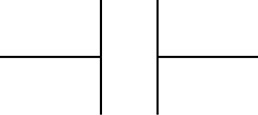
FIGURE 4.1 Schematic symbol for a non-polarized capacitor.
However, a capacitor does store an electron charge, which makes it like a battery that can quickly charge and discharge DC voltages. If the voltage is an AC signal, it can restrict or pass AC currents depending on its capacitance value, measured in micro farads, nano farads, or pico farads, which are all a fraction of a farad.
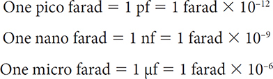
Here are some examples of equivalent capacitances:
• 100,000 pf = 100 nf = 0.1 μf
• 10,000 pf = 10 nf = 0.01 μf
• 1000 pf = 1 nf = 0.001 μf
For many capacitors, including ceramic and film type capacitors, the capacitance value is printed in the form of a first and second significant numerical digit and a third multiplier numerical digit, plus a fourth “digit” that is a letter (e.g., K = 10% or M = 20%) to denote the tolerance or accuracy of the capacitance value. The third digit can also be interpreted as the number of zeros after the first two digits.
In general, the three numerical digits tell us the capacitance value in pico farads, which you can equivalently express in nano or micro farads. See the examples below:
• 103 = 10 × 103 pf = 10,000 pf= 10 nf = 0.01 μf
• 185 = 18 × 105 pf = 1,800,000 pf (note the five zeros after the “18”), which is really more commonly expressed as 1.8 μf
• 101 = 10 × 101 = 10 × 10 = 100 pf and NOT 101 pf
• 270 = 27 × 100 = 27 × 1 = 27 pf and NOT 270 pf. However, sometimes a capacitor will be marked by its literal value, and 270 can equal 270 pf. This is why a DVM with a capacitance measurement feature comes in handy.
Many ceramic and film (e.g., polyester, mylar, polycarbonate, or polypropylene) capacitors include a letter to denote the accuracy or tolerance of the capacitance value. The most common letters used are the following list, and the most common tolerances for capacitors are highlighted in the bold fonts:
• M = ± 20%
• K = ± 10%
• J = ± 5%
• G = ± 2%
• F = ± 1%
• Z = –20% to +80
As an example, here is the capacitance range of a 1000 pf 10 percent capacitor, which is marked 102K:

Therefore, it is rare that the capacitor’s capacitance will be exactly as marked. For example, if you measure an off-the-shelf capacitor marked 2.2 μf, it will most likely read below or above that value on the capacitance meter.
Sometimes the capacitor is marked with a “K” after the third numerical digit, which may be confusing as to what the capacitance value really is. This is because the K may also mean kilo instead of 10 percent tolerance. See Figure 4-2.
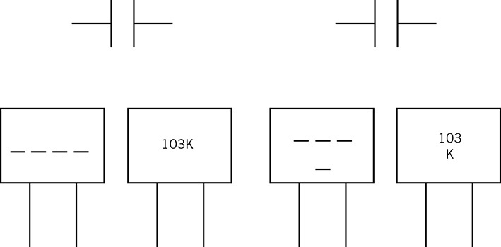
FIGURE 4.2 Capacitor symbols with typical markings either 4 consecutive “digits” on the left side, or 3 digits plus the tolerance letter below as shown on the right side.
On the left side the 0.01 μf (10,000 pf), 10 percent tolerance cap marked “103K” may be misinterpreted because K may be (incorrectly, in this case) thought of as equal to 1000. See examples A and B below, which are incorrect or misinterpreted:
103 × 1000 pf = 103,000 pf = 0.103 μf
or as:
10,000 pf × 1000 = 10 million pf = 10 μf
Again the correct value of a capacitor marked as 103K is a 0.01 μf (or 10 nf) capacitor with 10 percent tolerance.
Generally, for electronics work, a farad is too large a value, and capacitors that have capacitances in the 1-farad range are considered to be “super capacitors.” These super capacitors are used in some power supply filter circuits or as a battery to keep memory circuits working when power is cut off.
In many circuits, the capacitors are non-polarized, which means that you can connect them in any manner without worrying about the polarity of the DC voltage across them. For example, a non-polarized capacitor will work properly whether a negative or positive voltage is applied across it.
One of the major “problems” constructing circuits with capacitors is that these days they look “all the same.” In the past, it was easier to spot a larger value capacitor by just looking at the physical size. See Figure 4-3.
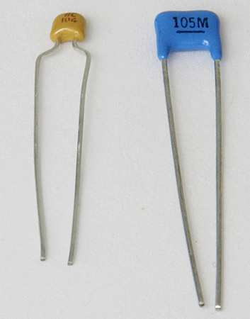
FIGURE 4.3 A smaller dimension 0.1 μf (104) capacitor on the left with large physical size 1 μf (105M = 1 μf at 20 percent tolerance) capacitor on the right side.
As we can see in Figure 4-3, we can easily spot the larger capacitance value capacitor by observing both capacitors’ dimensions.
However, with the advent of newer technology, capacitors of small and large values have “equal” sizes. Let’s look at ceramic capacitors that have essentially the same size for a very wide range of capacitances. See Figure 4-4.

FIGURE 4.4 Ceramic capacitors ranging from 10 pf to 10,000,000 pf (10 μf) that are essentially the same size.
In Figure 4-4, the capacitors from left to right are: 10 pf, 100 pf, 1000 pf, 100,000 pf (0.1 μf), 1,000,000 pf (1 μf), and lastly 10,000,000 pf (10 μf).
Because the capacitors of various values look the same size, I would recommend measuring the capacitance function on an appropriate multimeter. For example, see Figure 4-5.
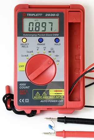
FIGURE 4.5 Measuring a 1 μf (105M) capacitor with an auto-ranging DVM that reads 0.897 μf.
In Figure 4-5, the 105M (1 μf 20 percent tolerance) capacitor shown on the right side of Figure 4-3 measures 0.897 μf, which is well within the 20 percent tolerance since a 1 μf 20 percent capacitor ranges from 0.8 μf to 1.2 μf. Also note that the capacitor is connected only to the test leads, and not to a circuit. When testing a capacitor, it should be out of the circuit. If you have to measure a capacitor in a circuit, first shut off the circuit by turning off the power supply or source, then remove one lead from the circuit and apply the test leads to the capacitor. This method works reasonably well for capacitor values > 1000 pf. For measuring smaller value capacitors < 1000 pf, it’s better to remove the capacitor from the circuit and measure the capacitor with a DVM that has a 2 nf (2000 pf) full scale range such as those shown in Chapter 3, Figure 3-7.
NOTE: Beware of large-value, small-sized capacitors with low working voltages; their capacitance can “depreciate” as more DC voltage is applied across them. For example, some ceramic capacitors may have half the rated capacitance at close to the maximum rated voltage.
We now turn to polarized capacitors that have positive and negative leads. When a polarized capacitor is in a circuit, the voltage across the positive to negative lead must read a positive value at all times. See Figure 4-6 on the schematic symbol.

FIGURE 4.6 A polarized capacitor’s schematic symbol with a curved or bent negative plate to distinguish it from a non-polarized capacitor symbol (Figure 4-1).
A polarized capacitor is usually reserved for larger values, and polarity must be observed. If the voltage across it is not the correct polarity, the capacitor can start drawing DC current and the capacitance value may drop. Worse yet, if the polarized capacitor is connected incorrectly polarity-wise, it may cause injury. As a safety issue, always check the wiring of a polarized capacitor before turning on the power. If there is a problem, rewire the polarized capacitor.
All polarized capacitors have a maximum voltage rating. In general, use a maximum voltage rating of twice the supply voltage if possible. For example, if you have a circuit that runs on 12 volts DC, the electrolytic capacitors should be rated at 25 volts. This 100 percent safety margin allows safe operation for any tolerance and surge voltages from the power supply. Also, the extra maximum voltage rating normally provides longer service life of the capacitor.
For example, if you have a 9-volt powered circuit and you put a 10-volt electrolytic capacitor across the 9-volt supply, chances are that this 10-volt capacitor will lose capacitance faster over time than if you used a 16-volt or 25-volt electrolytic capacitor.
Larger value capacitors from 0.1 μf to > 10,000 μf are generally polarized electrolytic capacitors. Generally polarized electrolytic capacitors have tolerances of ± 20 percent, or in some cases like the “Z” tolerance of –20 percent to +80 percent.
However, it is possible to purchase non-polarized electrolytic capacitors that range from 0.47 μf to 6800 μf. Non-polarized electrolytic capacitors are also known as bi-polarized or bi-polar electrolytic capacitors.
NOTE: You can make a non-polarized (NP) capacitor by connecting two equal value capacitance polarized capacitors back to back in series with the two negative terminals connected, or with the two positive terminals connected. The final capacitance is half of the value of one capacitor. See Figure 4-7.

FIGURE 4.7 Schematic symbols on the top row for regular, non-polarized (NP), and polarized capacitors, with examples on the bottom row on how to make a non-polarized capacitor with two polarized capacitors in series.
For example, if you connect two polarized 100 μf electrolytic capacitors in series back to back, the final capacitance will be half of 100 μf, or 50 μf.
Again often for electronics work, a farad or 1,000,000 μf is too large a value, and capacitors that have capacitances in the 1-farad range are considered to be “super capacitors.” These super capacitors are used in some power supply filter circuits in car audio systems, or as a battery backup DC voltage source to keep low current memory circuits working when the main power is turned off.
Radial and Axial Electrolytic Capacitors
When the two leads from the capacitor protrude from one side (e.g., bottom side), they are radial leaded types. See Figure 4-8 and note the polarity markings and their working voltage.
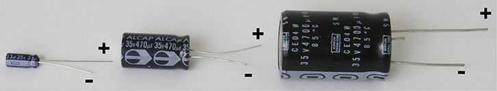
FIGURE 4.8 Radial lead capacitors at 33 μf, 470 μf, and 4700 μf, all at 35 volts maximum working voltage. Note the (–) stripes and that the negative leads are shorter than the positive leads.
Again, in an aluminum electrolytic capacitor, the negative lead is denoted by a stripe, usually with a minus sign (–).
When the capacitor has leads from both sides, it is an axial lead capacitor. See Figure 4-9.

FIGURE 4.9 A 100-μf, 16-volt axial lead electrolytic capacitor.
Note in the axial lead capacitor, there is an arrow that points to the negative lead. Often the negative lead is connected to the aluminum case.
Another way to identify the polarity is that the lead or wire from the insulated side is the positive lead. See Figure 4-10.
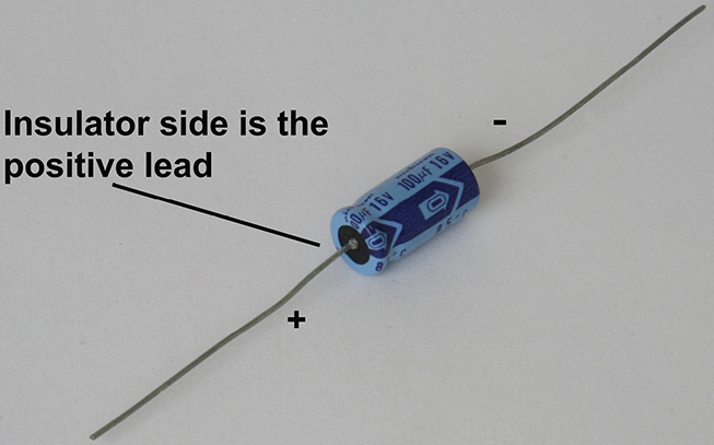
FIGURE 4.10 A view of the 100-μf, 16-volt electrolytic capacitor showing its positive lead.
Finally for this section, we will show how to make non-polarized electrolytic capacitors from polarized ones. See Figure 4-11.
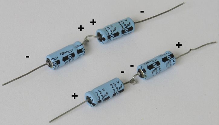
FIGURE 4.11 Examples of making non-polarized capacitors via a series connection.
As illustrated in Figure 4-7 schematically, we see in Figure 4-11 that two 3.3-μf electrolytic 25-volt capacitors are soldered in series back to back. In the top pair the two positive (+) leads are soldered. And in the bottom pair, the two negative (–) leads are connected. In both cases the result is a non-polarized capacitor whose capacitance is one-half of 3.3 μf or about 1.65 μf.
To be on the safe side, I would rate the maximum voltage at 25 volts and not 50 volts because there is no guarantee that the voltage is equal across each capacitor.
Measure Twice, Install Once: Erroneously Marked Capacitors
Once in a while, it is possible to run into an incorrectly marked capacitor. Figure 4-12 shows such an example.

FIGURE 4.12 A ceramic capacitor marked 684 = 0.68 μf reads instead 0.157 μf.
As we can see from Figure 4-12, the capacitor is marked 0.68 μf, but measures instead 0.157 μf. Thus, this 0.68-μf capacitor is mismarked or defective. In fact, it may be a 0.15-μf capacitor printed incorrectly.
A Proper Method for Measuring Capacitors
1. Measure the capacitor with a DVM or capacitance meter when the circuit is shut off and at least one of the capacitor’s leads is completely disconnected from the circuit. The DVM or capacitance meter sends out a signal to the capacitor during its measurement. Any “extraneous signal” added to the capacitor via being connected to the circuit will give erroneous capacitance readings, or worse, can cause damage to the DVM or capacitance meter.
2. Make sure to not touch either of the capacitor’s lead with your hands. For example, if you hold the capacitor with both hands to make the measurement, your hands can cause an erroneous measurement. This is true when you are measuring low capacitances such as 10 pf. Use alligator or EZ hook test leads to connect the capacitor to the DVM or capacitance meter.
3. If you are measuring low-value capacitances < 100 pf, then you must subtract off any residual capacitance reading from the DVM or capacitance meter. For example, take note of the capacitance read when the test capacitor is not connected. Usually, this residual capacitance will be in the < 2-pf range. Connect the capacitor and note the reading, and then subtract the residual capacitance. It’s very much like stepping on a bathroom scale that is not zeroed, such as it showing 5 pounds with no weight on it. You then step on the scale, look at the reading, and to get the true weight, you subtract 5 pounds in this example.
Resistors
Resistors restrict the flow of electric current. But they are used in many circuits to set up a DC voltage to an electronic component such as a transistor or integrated circuit. In other uses, resistors can be used to set the gain of an amplifier or set the voltage output of a DC power supply.
In terms of troubleshooting, the most common “error” in using resistors is mis-reading the color code on the resistor. In some cases, resistors come prepackaged with the resistance value, in ohms, which can be mismarked.
Back in the days before the Internet and apps, most people had to memorize the resistor color code to read the resistance value of the resistor. Today, one can learn the resistor color code, but it is easier to just measure it with the ohm meter that is in virtually all digital voltmeters. A resistor is measured in ohms and has a “shorthand” symbol using the Greek letter omega (Ω). So whenever you see Ω, it means ohm or ohms.
For example, instead of writing 120 ohms, we can equivalently restate it as 120Ω.
Figure 4-13 shows a drawing of a standard four-band (e.g., 5 percent tolerance) resistor.
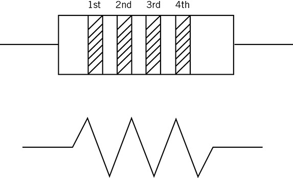
FIGURE 4.13 Standard tolerance four-band resistor and its associated schematic diagram symbol.
NOTE: A resistor is a non-polarized electronic component. Put another way, there are no polarities in resistors. Thus, you can connect their two leads to a circuit in any order.
To read the four-band resistor, we look at the first band, where the first band is located closer to the edge of the resistor than the fourth band. We start reading the resistor from first and second bands to get the first two digits, then read the third band to multiply by a number such as 0.01, 0.10, 1, 10, 100, 1000, etc. Sometimes people read the third band to add the number of zeroes after the first two digits.
Since each band is a color including black and white, let’s take a look at the code that is based on colors of the rainbow. The colors below are for the first, second and third band, but not the fourth band. Note that the third band denotes the number of zeroes after the first two digits. So if the third band is red, for example, it is not the number 2, but two zeroes added after the first two digits.
The fourth band represents the tolerance, which is either gold = 5 percent or silver = 10 percent. There are no other colors than these two for the fourth band.
For example, a 5600-ohm 5 percent tolerance resistor will show the following colors from first to fourth bands:
Green, blue, red, and gold
0 = black
1 = brown
2 = red
3 = orange
4 = yellow
5 = green
6 = blue
7 = violet
8 = gray
9 = white
Divide by 10 or multiply by 0.10 = gold
Divide by 100 or multiply by 0.01 = silver
When the third band has gold or silver “colors,” these are lower-value resistors (< 10Ω). For example, a 2.7Ω 5 percent resistor is denoted as red, violet, gold, and gold. And a 0.39Ω 5 percent resistor has its first to fourth bands as: orange, white, silver, and gold. See Figure 4-14 for examples of four-band color-coded resistors.
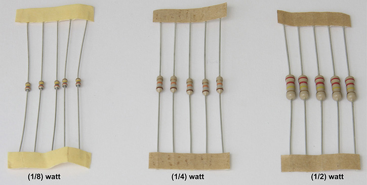
FIGURE 4.14 Four-band color-coded eighth-watt, quarter-watt, and half-watt resistors.
Five percent resistor values are incremented in about every 7 to 10 percent. For example, starting from a 220Ω resistor, the next value is 240Ω. If we want to have a 5 percent resistor that is in between, like 226Ω, there is no such value available because there are only two significant digits and “226” requires three significant digits.
Thus we need a resistor with five bands. The first three bands provide the three significant digits, the fourth band gives the number of zeroes, and the fifth band denotes the tolerance that is either brown for 1 percent tolerance, or red for 2 percent tolerance. More commonly, almost all five-band resistors have accuracy to within 1 percent with a brown fifth band. See Figure 4-15.
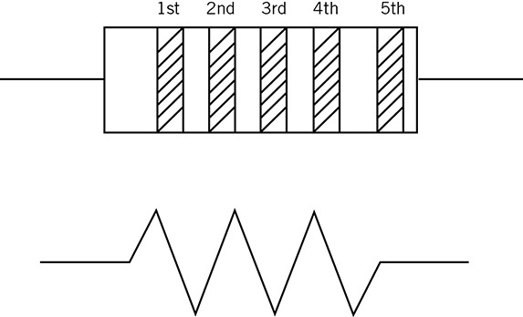
FIGURE 4.15 A five-band precision resistor with its schematic symbol below.
NOTE: There are some 2 percent five-band resistors where the fifth band is red.
Reading five-band resistors can be confusing because you have to look carefully to find where the first digit is. The first band is always a little bit farther from the edge of the resistor than the fifth band. The fifth band denotes the tolerance rating, which is usually brown for 1 percent. Note in Figure 4-14 the fifth band is almost right on the edge of the resistor, whereas the first band is not. Also notice that the spacing between the first four bands are the same, but the spacing is wider from the fourth to fifth bands.
Because the fifth band and the first band from far away may look the same distance from the end or edge of the resistor, you may have to read the resistor both left to right and right to left. Each reading will often give a different resistance value. So my recommendation is to take out your DVM and just measure the precision resistor in the ohm meter mode of the DVM. Figure 4-16 shows 5 percent and 1 percent resistors.
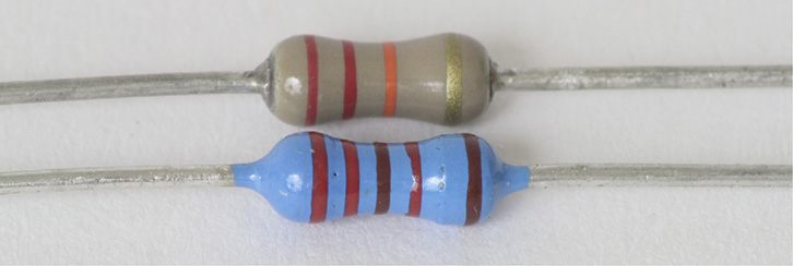
FIGURE 4.16 A 22KΩ, 5 percent resistor on the top and 22.1KΩ, 1 percent resistor on the bottom. Note that the fifth band that denotes tolerance rating is closest to the edge in the 1 percent resistor, and it has wider spacing between the adjacent fourth band.
Precision 1 percent resistors and even more accurate resistors with 0.5, 0.25, and 0.10 percent tolerances will have four numbers printed to determine the resistance value, followed by a letter to provide tolerance information. For example, the tolerance code is
F = 1 percent
D = 0.5 percent
C = 0.25 percent
B = 0.1 percent
A 1 percent 4750Ω resistor will read 4751F. Remember that the fourth number denotes the number of zeroes after the first three digits.
Another example having a 0.25 percent 10,000Ω resistor will read 1002B. That’s 100 + 2 zeroes afterward from the first 3 digits. This gives 10,000Ω or 10KΩ, where K is a thousand or 1000. See Figure 4-17.

FIGURE 4.17 From top to bottom: 226Ω 1 percent (F), 1000Ω 0.25 percent (C), and a 1000Ω 0.10 percent (B) precision resistors.
Using a DVM to Measure Resistance Values
Suppose we have a DVM whose maximum resistance ranges are:
• 200Ω
• 2000Ω
• 20kΩ
• 200kΩ
• 2000kΩ (or 2MΩ)
Which setting should we use to measure for the most accuracy for a 390Ω 5 percent (orange/white/brown/gold) resistor? The answer is the 2000Ω maximum resistance setting.
Before we measure resistance using a DVM, remember the following:
• Turn off the circuit’s power.
• Disconnect at least one resistor lead from the circuit.
Do not hold the resistor with the DVMs test probes/wires with both your hands. The resistance from your hands may give an erroneous lower resistance measurement. This is common when the resistance measurements are > 100kΩ. As a matter of fact, if you have sweaty hands or if the humidity is high in your area, then measuring a high resistance value (e.g., > 2000kΩ) will result in the DVM measuring your hand-to-hand resistance in combination with the resistor. This will result in a lower and inaccurate reading. You can hold one probe and one resistor lead together with one hand. And the insulated portion of the second probe is handled by the other hand while the metallic tip of the second probe touches the second resistor lead. You will now get an accurate reading without the DVM measuring your hand-to-hand resistance.
Now let’s take a look at measuring the 390Ω with all the resistance settings in the DVM. See Figures 4-18 to 4-22.
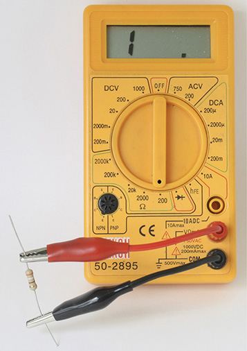
FIGURE 4.18 The 390Ω resistor shows a “1” and blank digits indicating “out of range” at the DVM’s 200Ω setting.
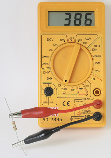
FIGURE 4.19 At the DVM’s 2000Ω setting we see a reading of 386Ω for the 390Ω resistor.
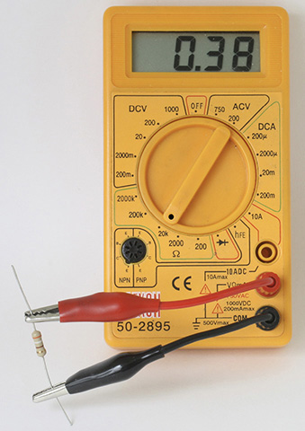
FIGURE 4.20 With the DVM’s 20kΩ setting, the DVM is displaying in kilo-ohms. The 390Ω resistor is measured as 0.38kΩ = 380Ω. Note that we just lost some accuracy compared to Figure 4-19, which measured 386Ω.

FIGURE 4.21 At the 200kΩ setting, the DVM is “looking” for resistors in the 10kΩ range. So the 390Ω resistor is measured as 0.3kΩ = 300Ω. Note that we are further losing measurement accuracy.
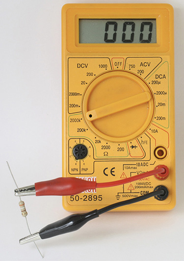
FIGURE 4.22 With the DVM’s resistance set to 2000kΩ or 2MΩ, it is expecting resistance values in the 100kΩ range. And with this setting it cannot resolve measuring resistances below 1000Ω. Any resistor value below 1000Ω, such as 390Ω, will register as zero as shown above.
One quick way to measure resistors without thinking too much is to turn the selector until you see the most significant digits displayed.
Measuring Low Resistance Values
In some cases, you will be measuring resistors that are less than 100Ω, such as 10Ω to 1Ω. What you will find in many DVMs is that the test leads may have resistances in the order of 1Ω. It depends on the length of the test leads, which can be short (< 2 inches) or longer (in the 2-foot range).
To make an accurate reading, touch the two test leads together to measure their resistance. Then measure the resistor, and to get the correct value, subtract the test leads’ resistance. See Figures 4-23 and 4-24.
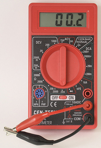
FIGURE 4.23 Shorting the test leads to read their resistance.
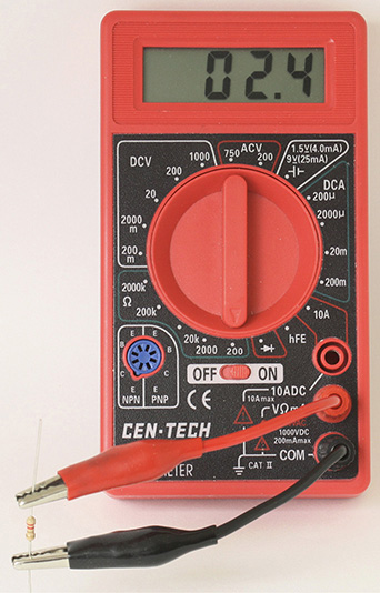
FIGURE 4.24 The combined test leads’ resistance (0.2Ω) with the 2.2Ω resistor is 2.4Ω.
In Figure 4-23 the test leads’ length is short. Normally, the standard test leads that come with a DVM are longer, and may exhibit resistances greater than 0.2Ω. However, if the test leads use heavy gauge wires, the leads may have < 0.2Ω.
Now we will measure a 2.2Ω resistor. See Figure 4-24.
To obtain the correct measurement of the resistor, subtract the test leads’ 0.2Ω from the 2.4Ω measurement in Figure 4-24. The answer is then:
2.4Ω − 0.2Ω = 2.2Ω
Note that in Figures 4-23 and 4-24, the test leads are very short. Standard test leads are generally 18 inches or more, which can exhibit more than 0.2Ω.
Some DVMs have a zero calibration mode, which subtracts out the test leads’ resistance. For example, in the Keysight U1232A DVM short or connect the two test leads together until the resistance value settles to a constant value such as 2.2Ω (or some other resistance value depending on the resistance of the test leads), keep the test leads connected or shorted together, then hit once the ΔNull/Recall button to zero out the resistance value of the test leads. You are now ready to measure resistances with the DVM calibrated.
NOTE: If you shut off the DVM and later turn it on, you should repeat the calibration procedure.
See Figure 4-25 for a picture of the Keysight U1232A DVM with ΔNull/Recall button.
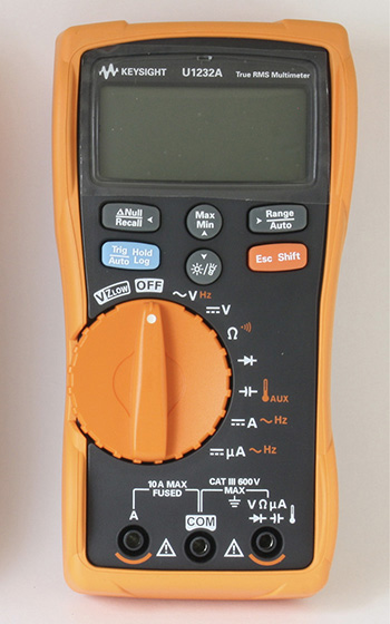
FIGURE 4.25 Keysight U1232A DVM with the ΔNull/Recall button and to the right of it, the Max Min key.
To calibrate and zero out the test leads’ resistance, first connect or short the two test leads until a resistance reading is stable. Then keep the two leads connected or shorted, and then hit/tap once the ΔNull/Recall button that is to the left of the Max Min key. You should now see zero ohms on the display with the test leads connected or shorted together.
We have now covered resistors and capacitors. In the next chapter we will examine semiconductors such as diodes, rectifiers, and zener diodes.