2
Probabilistic Approaches for Treating Uncertainty
Probability has been, and continues to be, a fundamental concept in the context of risk assessment. Unlike the other measures of uncertainty considered in this book, probability is a single-valued measure.
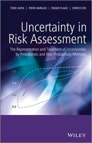
The common axiomatic basis of probability is found in Kolmogorov's (1933) probability axioms. Let ![]() denote events in a sample space
denote events in a sample space ![]() . The following probability axioms are assumed to hold:
. The following probability axioms are assumed to hold:
(2.1) 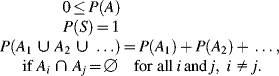
These axioms specify that probability is a non-negative, normalized, and additive measure.
Different types of operational or conceptual interpretations of probability can be distinguished. Among the most common are:
- Classical
- Relative frequency
- Subjective
- Logical.
Modern probability theory is not based on a particular interpretation of probability, although its standard language is best suited to the classical and relative frequency interpretations (Aven, 2012). In the context of risk assessment, the relative frequency and subjective interpretations are most common. Relative frequency probability is broadly recognized as the proper representation of variation in large populations (aleatory uncertainty), also among proponents of alternative representations of uncertainty; see, for example, Baudrit, Dubois, and Guyonnet (2006) and Ferson and Ginzburg (1996). The subjective interpretation, where probability is understood as expressing a degree of belief and measuring epistemic uncertainty, is also widely applied in risk assessment (Bedford and Cooke, 2001). The classical and logical interpretations of probability have less relevance in the context of risk assessment, as will be seen in the coming sections where we review and discuss the interpretations mentioned above. The review, which to a large extent is taken from or based on Aven (2013a), covers also the Bayesian subjective probability framework, which through the concept of chance provides a link between subjective probability and limiting relative frequencies.
2.1 Classical Probabilities
The classical interpretation of probability dates back to de Laplace (1812). It applies only in situations involving a finite number of outcomes which are equally likely to occur. The probability of an event ![]() is equal to the ratio between the number of outcomes resulting in
is equal to the ratio between the number of outcomes resulting in ![]() and the total number of possible outcomes, that is,
and the total number of possible outcomes, that is,
(2.2) ![]()
Consider as an example the tossing of a die. Then ![]() , as there are six possible outcomes which are equally likely to appear and only one outcome which gives the event that the die shows “1.” The requirement for each outcome to be equally likely is crucial for the understanding of this interpretation and has been subject to much discussion in the literature. A common perspective taken is that this requirement is met if there is no evidence favoring some outcomes over others. This is the so-called “principle of indifference,” also sometimes referred to as the “principle of insufficient reason.” In other words, classical probabilities are appropriate when the evidence, if there is any, is symmetrically balanced (Hajek, 2001), such as we may have when throwing a die or playing a card game.
, as there are six possible outcomes which are equally likely to appear and only one outcome which gives the event that the die shows “1.” The requirement for each outcome to be equally likely is crucial for the understanding of this interpretation and has been subject to much discussion in the literature. A common perspective taken is that this requirement is met if there is no evidence favoring some outcomes over others. This is the so-called “principle of indifference,” also sometimes referred to as the “principle of insufficient reason.” In other words, classical probabilities are appropriate when the evidence, if there is any, is symmetrically balanced (Hajek, 2001), such as we may have when throwing a die or playing a card game.
The classical interpretation is, however, not applicable in most real-life situations beyond random gambling and sampling, as we seldom have a finite number of outcomes which are equally likely to occur. The discussion about the principle of indifference is interesting from a theoretical point of view, but a probability concept based solely on this principle is not so relevant in a context where we search for a concept of probability that can be used in a wide range of applications.
2.2 Frequentist Probabilities
The frequentist probability of an event ![]() , denoted
, denoted ![]() , is defined as the fraction of times event
, is defined as the fraction of times event ![]() occurs if the situation/experiment considered were repeated (hypothetically) an infinite number of times. Thus, if an experiment is performed
occurs if the situation/experiment considered were repeated (hypothetically) an infinite number of times. Thus, if an experiment is performed ![]() times and event
times and event ![]() occurs
occurs ![]() times out of these, then
times out of these, then ![]() is equal to the limit of
is equal to the limit of ![]() as
as ![]() tends to infinity (tacitly assuming that the limit exists), that is,
tends to infinity (tacitly assuming that the limit exists), that is,
(2.3) ![]()
Taking a sample of repetitions of the experiment, event ![]() occurs in some of the repetitions and not in the rest. This phenomenon is attributed to “randomness,” and asymptotically the process generates a fraction of successes, the “true” probability
occurs in some of the repetitions and not in the rest. This phenomenon is attributed to “randomness,” and asymptotically the process generates a fraction of successes, the “true” probability ![]() , which describes quantitatively the aleatory uncertainty (i.e., variation) about the occurrence of event
, which describes quantitatively the aleatory uncertainty (i.e., variation) about the occurrence of event ![]() . In practice, it is of course not possible to repeat a situation an infinite number of times. The probability
. In practice, it is of course not possible to repeat a situation an infinite number of times. The probability ![]() is a model concept used as an approximation to a real-world setting where the population of units or number of repetitions is always finite. The limiting fraction
is a model concept used as an approximation to a real-world setting where the population of units or number of repetitions is always finite. The limiting fraction ![]() is typically unknown and needs to be estimated by the fraction of occurrences of
is typically unknown and needs to be estimated by the fraction of occurrences of ![]() in the finite sample considered, producing an estimate
in the finite sample considered, producing an estimate ![]() .
.
A frequentist probability is thus a mind-constructed quantity – a model concept founded on the law of large numbers which says that frequencies ![]() converge to a limit under certain conditions: that is, the probability of event
converge to a limit under certain conditions: that is, the probability of event ![]() exists and is the same in all experiments, and the experiments are independent. These conditions themselves appeal to probability, generating a problem of circularity. One approach to deal with this problem is to assign the concept of probability to an individual event by embedding the event into an infinite class of “similar” events having certain “randomness” properties (Bedford and Cooke, 2001, p. 23). This leads to a somewhat complicated framework for understanding the concept of probability; see the discussion in van Lambalgen (1990). Another approach, and a common way of looking at probability, is to simply assume the existence of the probability
exists and is the same in all experiments, and the experiments are independent. These conditions themselves appeal to probability, generating a problem of circularity. One approach to deal with this problem is to assign the concept of probability to an individual event by embedding the event into an infinite class of “similar” events having certain “randomness” properties (Bedford and Cooke, 2001, p. 23). This leads to a somewhat complicated framework for understanding the concept of probability; see the discussion in van Lambalgen (1990). Another approach, and a common way of looking at probability, is to simply assume the existence of the probability ![]() , and then refer to the law of large numbers to give
, and then refer to the law of large numbers to give ![]() the limiting relative frequency interpretation. Starting from Kolmogorov's axioms (as in the second paragraph of the introduction to Part II; see also Bedford and Cooke 2001, p. 40) and the concept of conditional probability, as well as presuming the existence of probability, the theory of probability is derived, wherein the law of large numbers constitutes a key theorem which provides the interpretation of the probability concept.
the limiting relative frequency interpretation. Starting from Kolmogorov's axioms (as in the second paragraph of the introduction to Part II; see also Bedford and Cooke 2001, p. 40) and the concept of conditional probability, as well as presuming the existence of probability, the theory of probability is derived, wherein the law of large numbers constitutes a key theorem which provides the interpretation of the probability concept.
The so-called propensity interpretation is yet another way of justifying the existence of a probability (SEP, 2009). This interpretation specifies that probability should primarily be thought of as a physical characteristic: The probability is a propensity of a repeatable experimental set-up which produces outcomes with limiting relative frequency ![]() . Consider as an example a coin. The physical characteristics of the coin (weight, center of mass, etc.) are such that when tossing the coin over and over again the fraction of heads will be p (Figure 2.1). The literature on probability shows that the existence of a propensity is controversial (Aven, 2013a). However, from a conceptual point of view the idea of a propensity may be no more difficult to grasp than the idea of an infinite number of repetitions of experiments. If the framework of frequentist probability is accepted, that is, if referring to an infinite sequence of similar situations makes sense, the propensity concept should also be accepted as it essentially expresses that such a framework exists.
. Consider as an example a coin. The physical characteristics of the coin (weight, center of mass, etc.) are such that when tossing the coin over and over again the fraction of heads will be p (Figure 2.1). The literature on probability shows that the existence of a propensity is controversial (Aven, 2013a). However, from a conceptual point of view the idea of a propensity may be no more difficult to grasp than the idea of an infinite number of repetitions of experiments. If the framework of frequentist probability is accepted, that is, if referring to an infinite sequence of similar situations makes sense, the propensity concept should also be accepted as it essentially expresses that such a framework exists.
Figure 2.1 Repetition of the experiment of tossing a coin.
Thus, for gambling situations and when dealing with fractions in large populations of similar items, the frequentist probability concept makes sense, as a model concept. Of course, if a die is thrown over and over again a very large number of times its physical properties will eventually change, so the idea of “similar experiments” is questionable. Nevertheless, for all practical purposes we can carry out (in theory) a large number of trials, say 100 000, without any physical changes in the experimental set-up, and that is what is required for the concept to be meaningful. The same is true if we consider a population of (say) 100 000 human beings belonging to a specific category, say men in the age range 20 to 30 years old in a specific country.
It is not surprising, then, that frequency probabilities are so commonly and widely adopted in practice. The theoretical concept of a frequentist probability is introduced, often in the form of a probability model – for example, the binomial, normal (Gaussian), or Poisson distributions – and statistical analysis is carried out to estimate the frequentist probabilities (more generally the parameters of the probability models) and to study the properties of the estimators using well-established statistical theory. However, the types of situations that are captured by this framework are limited. As noted by Singpurwalla (2006, p. 17), the concept of frequency probabilities “is applicable to only those situations for which we can conceive of a repeatable experiment.” This excludes many situations and events. Consider for example events such as the rise of sea level over the next 20 years, the guilt or innocence of an accused individual, or the occurrence or not of a disease in a specific person with a specific history.
What does it mean that the situations under consideration are “similar?” The “experimental conditions” cannot be identical, since we would then observe exactly the same outcome and the ratio ![]() would be either 1 or 0. What kind of variation between the experiments is allowed? This is often difficult to specify and makes it challenging to extend frequentist probabilities to include real-life situations. Consider as an example the frequentist probability that a person
would be either 1 or 0. What kind of variation between the experiments is allowed? This is often difficult to specify and makes it challenging to extend frequentist probabilities to include real-life situations. Consider as an example the frequentist probability that a person ![]() contracts a specific disease
contracts a specific disease ![]() . What should be the population of similar persons in this situation? If we include all men/women of his/her age group we get a large population, but many of the people in this population may not be very “similar” to person
. What should be the population of similar persons in this situation? If we include all men/women of his/her age group we get a large population, but many of the people in this population may not be very “similar” to person ![]() . We may reduce the population to increase the similarity, but not too much as that would make the population very small and hence inadequate for defining the frequentist probability. This type of dilemma is faced in many types of modeling and a balance has to be made between different concerns: similarity (and hence relevance) vs. population size (and hence validity of the frequentist probability concept, as well as data availability).
. We may reduce the population to increase the similarity, but not too much as that would make the population very small and hence inadequate for defining the frequentist probability. This type of dilemma is faced in many types of modeling and a balance has to be made between different concerns: similarity (and hence relevance) vs. population size (and hence validity of the frequentist probability concept, as well as data availability).
2.3 Subjective Probabilities
The theory of subjective probability was proposed independently and at about the same time by Bruno de Finetti in Fondamenti Logici del Ragionamento Probabilistico (de Finetti, 1930) and Frank Ramsey in The Foundations of Mathematics (Ramsey, 1931); see Gillies (2000).
A subjective probability – sometimes also referred to as a judgmental or knowledge-based probability – is a purely epistemic description of uncertainty as seen by the assigner, based on his or her background knowledge. In this view, the probability of an event ![]() represents the degree of belief of the assigner with regard to the occurrence of
represents the degree of belief of the assigner with regard to the occurrence of ![]() . Hence, a probability assignment is a numerical encoding of the state of knowledge of the assessor, rather than a property of the “real world.”
. Hence, a probability assignment is a numerical encoding of the state of knowledge of the assessor, rather than a property of the “real world.”
It is important to appreciate that, irrespective of interpretation, any subjective probability is considered to be conditional on the background knowledge ![]() that the assignment is based on. They are “probabilities in the light of current knowledge” (Lindley, 2006). This can be written as
that the assignment is based on. They are “probabilities in the light of current knowledge” (Lindley, 2006). This can be written as ![]() , although the writing of
, although the writing of ![]() is normally omitted as the background knowledge is usually unmodified throughout the calculations. Thus, if the background knowledge changes, the probability might also change. Bayes' theorem (see Section 2.4) is the appropriate formal tool for incorporating additional knowledge into a subjective probability. In the context of risk assessment, the background knowledge typically and mainly includes data, models, expert statements, assumptions, and phenomenological understanding.
is normally omitted as the background knowledge is usually unmodified throughout the calculations. Thus, if the background knowledge changes, the probability might also change. Bayes' theorem (see Section 2.4) is the appropriate formal tool for incorporating additional knowledge into a subjective probability. In the context of risk assessment, the background knowledge typically and mainly includes data, models, expert statements, assumptions, and phenomenological understanding.
There are two common interpretations of a subjective probability, one making reference to betting and another to a standard for measurement. The betting interpretation and related interpretations dominate the literature on subjective probabilities, especially within the fields of economy and decision analysis, whereas the standard for measurement is more common among risk and safety analysts.
2.3.1 Betting Interpretation
If derived and interpreted with reference to betting, the probability of an event ![]() , denoted
, denoted ![]() , equals the amount of money that the person assigning the probability would be willing to bet if a single unit of payment were given in return in case event
, equals the amount of money that the person assigning the probability would be willing to bet if a single unit of payment were given in return in case event ![]() were to occur, and nothing otherwise. The opposite must also hold: that is, the assessor must be willing to bet the amount
were to occur, and nothing otherwise. The opposite must also hold: that is, the assessor must be willing to bet the amount ![]() if a single unit of payment were given in return in case
if a single unit of payment were given in return in case ![]() were not to occur, and nothing otherwise. In other words, the probability of an event is the price at which the person assigning the probability is neutral between buying and selling a ticket that is worth one unit of payment if the event occurs and worthless if not (Singpurwalla, 2006). The two-sidedness of the bet is important in order to avoid a so-called Dutch book, that is, a combination of bets (probabilities) that the assigner would be committed to accept but which would lead him or her to a sure loss (Dubucs, 1993). A Dutch book can only be avoided by making so-called coherent bets, meaning bets that can be shown to obey the set of rules that probabilities must obey. In fact, the rules of probability theory can be derived by taking the avoidance of Dutch books as a starting point (Lindley, 2000).
were not to occur, and nothing otherwise. In other words, the probability of an event is the price at which the person assigning the probability is neutral between buying and selling a ticket that is worth one unit of payment if the event occurs and worthless if not (Singpurwalla, 2006). The two-sidedness of the bet is important in order to avoid a so-called Dutch book, that is, a combination of bets (probabilities) that the assigner would be committed to accept but which would lead him or her to a sure loss (Dubucs, 1993). A Dutch book can only be avoided by making so-called coherent bets, meaning bets that can be shown to obey the set of rules that probabilities must obey. In fact, the rules of probability theory can be derived by taking the avoidance of Dutch books as a starting point (Lindley, 2000).
Consider the event ![]() , defined as the occurrence of a specific type of nuclear accident. Suppose that a person specifies the subjective probability
, defined as the occurrence of a specific type of nuclear accident. Suppose that a person specifies the subjective probability ![]() . Then, according to the betting interpretation, this person is expressing that he/she is indifferent between:
. Then, according to the betting interpretation, this person is expressing that he/she is indifferent between:
- receiving (paying) €0.005; and
- taking a gamble in which he/she receives (pays) €1 if
 occurs and €0 if
  does not occur.
If the unit of money is €1000, the interpretation would be that the person is indifferent between:
- receiving (paying) €5; and
- taking a gamble where he/she receives (pays) €1000 if
 occurs and €0 if
  does not occur.
In practice, the probability assignment would be carried out according to an iterative procedure in which different gambles are compared until indifference is reached. However, as noted by Lindley (2006) (see also Cooke, 1986), receiving the payment in the nuclear accident example would be trivial if the accident were to occur (the assessor might not be alive to receive it). The problem is that there is a link between the probability assignment and value judgments about money (the price of the gamble) and the situation (the consequences of the accident). This value judgment has nothing to do with the uncertainties per se, or the degree of belief in the occurrence of event ![]() .
.
2.3.2 Reference to a Standard for Uncertainty
A subjective probability can also be understood in relation to a standard for uncertainty, for example, making random withdrawals from an urn. If a person assigns a probability of 0.1 (say) to an event ![]() , then this person compares his/her uncertainty (degree of belief) in the occurrence of
, then this person compares his/her uncertainty (degree of belief) in the occurrence of ![]() to drawing a specific ball from an urn containing 10 balls. The uncertainty (degree of belief) is the same. More generally, the probability
to drawing a specific ball from an urn containing 10 balls. The uncertainty (degree of belief) is the same. More generally, the probability ![]() is the number such that the uncertainty about the occurrence of
is the number such that the uncertainty about the occurrence of ![]() is considered equivalent, by the person assigning the probability, to the uncertainty about the occurrence of some standard event, for example, drawing, at random, a red ball from an urn that contains
is considered equivalent, by the person assigning the probability, to the uncertainty about the occurrence of some standard event, for example, drawing, at random, a red ball from an urn that contains ![]() red balls (see, e.g., Lindley, 2000, 2006; Bernardo and Smith, 1994).
red balls (see, e.g., Lindley, 2000, 2006; Bernardo and Smith, 1994).
As for the betting interpretation, the interpretation with reference to an uncertainty standard can be used to deduce the rules of probability; see Lindley (2000). These rules are typically referred to as axioms in textbooks on probability, but they are not axioms here, since they are deduced from more basic assumptions linked to the uncertainty standard; see Lindley (2000, p. 299). Whether the probability rules are deduced or taken as axioms may not be so important to applied probabilists. The main point is that these rules apply, and the uncertainty standard provides an easily understandable way of defining and interpreting subjective probability where uncertainty/probability and utility/value are separated. The rules of probability reduce to the rules governing proportions, which are easy to communicate.
2.4 The Bayesian Subjective Probability Framework
The so-called Bayesian framework has subjective probability as a basic component, and the term “probability” is reserved for, and always understood as, a degree of belief. Within this framework, the term “chance” is used by some authors (e.g., Lindley, 2006; Singpurwalla, 2006; Singpurwalla and Wilson, 2008) for the limit of a relative frequency in an exchangeable, infinite Bernoulli series. A chance distribution is the limit of an empirical distribution function (Lindley, 2006). Two random quantities ![]() and
and ![]() are said to be exchangeable if for all values
are said to be exchangeable if for all values ![]() and
and ![]() that
that ![]() and
and ![]() may take, we have
may take, we have
(2.5) ![]()
That is, the probabilities remain unchanged (invariant) when switching (permuting) the indices. The relationship between subjective probability and the chance concept is given by the so-called representation theorem of de Finetti; see, for example, Bernardo and Smith (1994, p. 172). Roughly speaking, this theorem states that if an exchangeable Bernoulli series can be introduced, one may act as though frequency probabilities exist.
In the case when a chance ![]() of an event
of an event ![]() may be introduced, we have
may be introduced, we have ![]() . That is, the probability of an event
. That is, the probability of an event ![]() for which the associated chance is known is simply equal to the value of the chance. For unknown
for which the associated chance is known is simply equal to the value of the chance. For unknown ![]() , observations of outcomes in similar (exchangeable) situations would not be considered independent of the situation of interest, since the observations would provide more information about the value of
, observations of outcomes in similar (exchangeable) situations would not be considered independent of the situation of interest, since the observations would provide more information about the value of ![]() . On the other hand, for known
. On the other hand, for known ![]() the outcomes would be judged as independent, since nothing more could be learned about
the outcomes would be judged as independent, since nothing more could be learned about ![]() from additional observations. Hence, conditional on
from additional observations. Hence, conditional on ![]() , the outcomes are independent, but unconditionally they are not – they are exchangeable. In practice, the value of a chance
, the outcomes are independent, but unconditionally they are not – they are exchangeable. In practice, the value of a chance ![]() is in most cases unknown and the assessor expresses his or her uncertainty about the value of
is in most cases unknown and the assessor expresses his or her uncertainty about the value of ![]() by a probability distribution
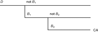
by a probability distribution ![]() . As in the example of Section 1.1.3, the probability of
. As in the example of Section 1.1.3, the probability of ![]() can then be derived as
can then be derived as
The probability ![]() in this equation characterizes uncertainty about the occurrence of event A, given the background knowledge
in this equation characterizes uncertainty about the occurrence of event A, given the background knowledge ![]() (suppressed from the notation), which includes a judgment of exchangeability which allows for the equivalence relation
(suppressed from the notation), which includes a judgment of exchangeability which allows for the equivalence relation ![]() , as well as the information contained in
, as well as the information contained in ![]() . Consequently, the uncertainty about p does not make
. Consequently, the uncertainty about p does not make ![]() uncertain.
uncertain.
More generally, if a chance distribution is known, then under judgment of exchangeability the probability distribution is equal to the chance distribution, which is analogous to setting ![]() . If the chance distribution is unknown, a “prior” probability distribution is established over the chance distribution (parameters), updated to a “posterior” distribution upon receiving new information, and the “predictive” probability distribution may be established by using the law of total probability, as illustrated in (2.6). The updating is performed using Bayes' rule, which states that
. If the chance distribution is unknown, a “prior” probability distribution is established over the chance distribution (parameters), updated to a “posterior” distribution upon receiving new information, and the “predictive” probability distribution may be established by using the law of total probability, as illustrated in (2.6). The updating is performed using Bayes' rule, which states that
(2.7) ![]()
for ![]() .
.
2.5 Logical Probabilities
Logical probabilities were first proposed by Keynes (1921) and later taken up by Carnap (1922, 1929). The idea is that probability expresses an objective logical relation between propositions – a sort of “partial entailment.” There is a number in the interval ![]() , denoted
, denoted ![]() , which measures the objective degree of logical support that evidence E gives to hypothesis
, which measures the objective degree of logical support that evidence E gives to hypothesis ![]() (Franklin, 2001). As stated by Franklin (2001), this view on probability has an intuitive initial attractiveness in representing a level of agreement found when scientists, juries, actuaries, and so on evaluate hypotheses in the light of evidence. However, as described by Aven (2013a), the notion of partial entailment has never received a satisfactory interpretation, and also both Cowell et al. (1999) and Cooke (2004) conclude that this interpretation of probability cannot be justified.
(Franklin, 2001). As stated by Franklin (2001), this view on probability has an intuitive initial attractiveness in representing a level of agreement found when scientists, juries, actuaries, and so on evaluate hypotheses in the light of evidence. However, as described by Aven (2013a), the notion of partial entailment has never received a satisfactory interpretation, and also both Cowell et al. (1999) and Cooke (2004) conclude that this interpretation of probability cannot be justified.