9
Uncertainty Representation and Propagation in Maintenance Performance Assessment
In this chapter, we consider the problem of uncertainty representation and propagation in the context of maintenance performance assessment. The application is in part based on Baraldi, Compare, and Zio (2012) and Baraldi, Compare, and Zio (2013a).
9.1 Maintenance Performance Assessment
In the last few decades, the relevance of maintenance in several sectors of industry has increased in influence on both productivity and safety. For example, maintenance represents a major portion of the total production cost of non-fossil-fuel energy production plants (nuclear, solar, wind, etc.) and its optimization is fundamental for the economic competitiveness of such plants (Zio and Compare, 2013).
In general, the goal of effective maintenance planning is the optimization of production and plant availability, in a way that guarantees safety and respects the associated regulatory requirements (Zio, 2009). For this, several approaches to maintenance modeling, optimization, and management have been proposed in the literature. Usually, these approaches are divided into two main groups: corrective maintenance and scheduled maintenance.
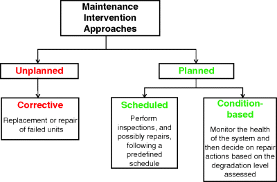
Under the corrective maintenance strategy, the components are operated until failure; then, repair or renovation actions are performed. This is the oldest approach to maintenance and is nowadays still adopted in some industries, especially for equipment which is neither safety critical nor crucial for the production performance of the plant, and whose spare parts are readily available and not expensive (Zio and Compare, 2011). Under some strategies, maintenance is performed on a scheduled basis, which can be predefined (periodic maintenance) or based on information on the degradation state of the equipment (condition-based maintenance). Figure 9.1 shows a sketch of the different maintenance approaches.
Figure 9.1 Maintenance intervention approaches (based on Baraldi, Zio, and Popescu, 2008).
In practice, the definition of a proper maintenance plan requires the following (Zio, 2009):
In this section, we focus on issues 2 and 3, taking into account the fact that the models developed for this aim typically rely on a number of parameters which are often weakly known in real applications. This is mainly due to the lack of real/field data collected during operation or properly designed tests. In these cases, the main source of information for estimating these parameters is experts' judgment.
9.2 Case Study
We consider the definition of a maintenance plan for a check valve of a turbo pump lubricating system in a nuclear power plant (Zille et al., 2009). This component undergoes one principal degradation mechanism, namely, fatigue, and only one failure mode, namely, rupture. The degradation process is modeled as a discrete-state, continuous-time stochastic process which evolves among the following three degradation levels (Figure 9.2):
- “Good”: A component in this state is new or almost new (no crack is detectable by maintenance operators).
- “Medium”: If the component is in this degradation state, then it is best to replace it.
- “Bad”: A component in this degradation state is very likely to experience a failure in a few working hours.
Figure 9.2 Degradation model based on a Petri net description.
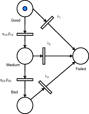
A further state, “Failed,” can be reached from every degradation state upon the occurrence of a shock event.
The choice of describing the degradation process by means of a small number of levels, or degradation “macro-states,” is driven by industrial practice: experts usually adopt a discrete and qualitative classification of the degradation states based on qualitative interpretations of symptoms.
This model of the degradation process can be represented by introducing the following five aleatory quantities:
 the transition time from degradation level “Good” to degradation level “Medium”
 the transition time from degradation level “Medium” to degradation level “Bad”
 the transition time from degradation level “Good” to the failed state
 the transition time from degradation level “Medium” to the failed state
 the transition time from degradation level “Bad” to the failed state.
A condition-based maintenance (CBM) approach is applied to the component. In practice, the component is periodically inspected by a plant operator according to a predefined schedule, and if during the inspection it is found in the degradation level “Medium” or “Bad,” it is replaced. Replacement is also performed after component failure. The following duration and costs, in arbitrary units due to the confidentiality of the data, are assumed for the different maintenance tasks:
- Inspections: These actions aim at detecting the degradation state of the component. Inspections, which are performed periodically on the basis of a predefined schedule, are assumed to last 5 h and have an associated cost of €50.
- Replacement after inspection: These actions are performed only if the component is found in the degradation states “Medium” or “Bad” during the inspection and consist of the preventive replacement of the degraded component. The replacement is assumed to last for 25 h and costs €500. After replacement, the component is set back to the “Good” degradation level.
- Replacement after failure: The corrective action is performed after component failure and consists of replacement of the failed component. Its duration is assumed to be 100 h and its cost €3500. The time necessary for replacement after failure is longer than that necessary for a preventive replacement performed after inspections, to take into account the time elapsing between the occurrence of the failure and the start of the replacement action and the extra time needed to repair other plant components which may be damaged by the component failure. Similarly, the replacement costs after failure also are higher than those after an inspection.
Under this approach, the only quantity to be decided by the maintenance planner to fully define the maintenance policy is the time span between two successively planned inspections, which will be referred to as the inspection interval II. The maintenance planner wants to find an optimal value of II with respect to his or her performance objectives such as safety, cost reduction, and availability. In this section, we assume that the planner is interested in the following maintenance performance indicators: (i) the maintenance costs and (ii) the component downtime over its mission time. In this context, two different types of uncertainty have to be considered for the assessment of the maintenance performance indicators:
- the stochasticity of the degradation and failure process;
- the epistemic uncertainty on the parameters of the probability distributions representing the transition and failure times.
In practice, we consider a model whose input quantities are the transition and failure times, and whose output quantities are the maintenance costs and the portion of downtime over the mission time. Note that the maintenance planner is interested in the expected values of these two uncertain quantities, which will be referred to as expected maintenance costs and average unavailability over the mission time. Since the outcomes of the input quantities are subject to aleatory uncertainty described by frequentist probabilities with parameters subject to epistemic uncertainty, uncertainty propagation requires a level 2 setting (Section 6.2).
 the transition time from degradation level “Good” to degradation level “Medium”
 the transition time from degradation level “Medium” to degradation level “Bad”
 the transition time from degradation level “Good” to the failed state
 the transition time from degradation level “Medium” to the failed state
 the transition time from degradation level “Bad” to the failed state
- parameters
 of the probability distribution representing the uncertainty on
- parameters
 of the probability distribution representing the uncertainty on
- parameter
 of the probability distribution representing the uncertainty on
- parameter
 of the probability distribution representing the uncertainty on
  .
.
- portion
 of the mission time in which the component is unavailable
 - maintenance costs,

- aleatory on

- epistemic on
 .
.
- level 2.
9.3 Uncertainty Representation
The representation of the uncertainty of the model input quantities, that is, the transition and failure times, ![]() , requires one to choose the probability distribution types and set their parameters.
, requires one to choose the probability distribution types and set their parameters.
In the context of degradation modeling, the Weibull distribution is commonly applied in fracture mechanics, especially under the weakest-link assumption (Remy et al., 2010) to represent transition times between degradation states. Thus, the transition times are represented by Weibull distributions characterized by uncertain scale and shape parameters, ![]() and
and ![]() , respectively, for the transitions from state
, respectively, for the transitions from state ![]() toward state
toward state ![]() (
(![]() and
and ![]() ).
).
With respect to failure times ![]() , their uncertainty has been represented using exponential distributions with constant failure rate
, their uncertainty has been represented using exponential distributions with constant failure rate ![]() , for every
, for every ![]() . The choice of using constant failure rates is driven by industrial practice: experts are familiar with this setting and comfortable with providing information about the failure rate values.
. The choice of using constant failure rates is driven by industrial practice: experts are familiar with this setting and comfortable with providing information about the failure rate values.
All the parameters of the distributions that model the transitions of the component among the four states of Figure 9.2 are not well known, and their evaluation comes (with imprecision) from teams of experts. With respect to the estimate of the parameters of the Weibull distributions, note that the scale parameter represents the time up to which almost 65% of the components have experienced the transition, and the shape parameters, the slopes of the Weibull probability plots. To sum up, the uncertainty situation is as follows. There are five stochastic uncertain quantities, which define the five transition times as given in Table 9.1. The distributions associated with the variables are known, and depend on a set of seven epistemic uncertain parameters, which are the shape and scale parameters of the two Weibull distributions and the failure rates pertaining to the three degradation levels.
Table 9.1 Model parameters.
| Random variables | Uncertain parameters | Description |
| Transition time from degradation level “Good” to “Medium” | ||
| Transition time from degradation level “Medium” to “Bad” | ||
| Transition time from degradation level “Good” to “Failed” | ||
| Transition time from degradation level “Medium” to “Failed” | ||
| Transition time from degradation level “Bad” to “Failed” |
However, the uncertainty on the third failure rate is not considered. In fact, a sensitivity analysis carried out by Baraldi, Compare, and Zio (2013a) has shown that the output of the model does not appreciably change when the value of the third failure rate varies over a wide interval, whereas accounting for a further uncertain parameter strongly increases the computational effort.
We assume that for each uncertain parameter, three experts are involved in the assessment of its value. Each expert is asked to provide the extreme values of the interval that he or she believes contain the true value of the uncertain parameter. The intervals provided by the three experts are given in Table 9.2. The generic interval will be referred to as ![]() , with
, with ![]() indicating the expert,
indicating the expert, ![]() , the stochastic transition or failure time, and
, the stochastic transition or failure time, and ![]() , the parameter of the probability distribution describing the transition or failure time (
, the parameter of the probability distribution describing the transition or failure time (![]() and
and ![]() ).
).
Table 9.2 Uncertainty ranges for the parameters provided by three independent sources.
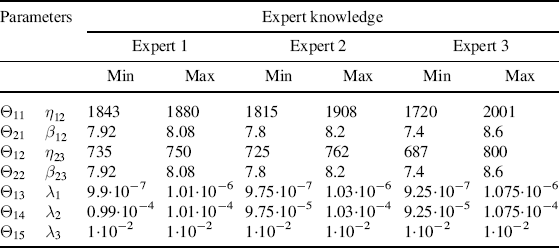
According to Section 6.2.2, the information elicited from the experts has been used to build, for each uncertain parameter ![]() ,
, ![]() and
and ![]() , an evidence space
, an evidence space ![]() . The domain of the parameter
. The domain of the parameter ![]() , that is, the set of its possible values, is the union of the three intervals provided by the experts,
, that is, the set of its possible values, is the union of the three intervals provided by the experts, ![]() , whereas the set of focal elements
, whereas the set of focal elements ![]() is made up of these three intervals. Finally, the BBA assigns to each interval the same mass value
is made up of these three intervals. Finally, the BBA assigns to each interval the same mass value
![]()
9.4 Uncertainty Propagation
The main quantities in which the maintenance decision makers are interested are the portion of downtime in the whole mission time and the cost associated with the maintenance policy. Since both quantities are uncertain, the decision maker typically considers their expected values, that is, the mean value of the portion of downtime in the whole mission time, which is indicated by the average unavailability over the mission time, EU, and the expected costs, EC.
In order to aid the reader's comprehension of this case study, in the next we present the uncertainty propagation results obtained in the unrealistic case of no epistemic uncertainty on the probability distribution parameters, whereas in Section 9.4.2 we describe the application of the hybrid probabilistic–theory of evidence uncertainty propagation method for this case study, in the situation where all sources of uncertainty are considered.
9.4.1 Maintenance Performance Assessment in the Case of no Epistemic Uncertainty on the Parameters
Table 9.3 lists the values used for the parameters of the failure and degradation time probability distributions, which have been taken from Zille et al. (2009) and correspond to the middle point of the intervals provided by the experts (Table 9.2). In this case, propagation of the uncertainty is performed within a level 1 uncertainty propagation setting and requires the application of the Monte Carlo (MC) method (Baraldi, Compare, and Zio, 2013b).
Table 9.3 Parameters of the probability distributions.
| Parameters | Nominal values |
| 1861 h | |
| 8 | |
| 743 h | |
| 8 | |
| 10−6 h−1 | |
| 10−4 h−1 | |
| 10−2 h−1 |
Each trial of a Monte Carlo simulation consists of generating a random walk that guides the component from one state to another, at different times. During a trial, starting from the state “Good” at time 0, we need to determine when the next transition occurs and what new state is reached by the system after the transition. The procedure, then, repeats until the time reaches the mission time. The time is suitably discretized in intervals, “bins,” and counters are introduced to accumulate the contributions to unavailability. In each counter, we accumulate the time in which the component has been unavailable, that is, in the state “failed,” during the bin. After all the MC histories have been performed, the content of each counter divided by the bin lengths and by the number of histories gives an estimate of the average unavailability of the component in that bin, and the average of all the obtained unavailability in the different bins gives the average unavailability of the component over the mission time. Note that this procedure corresponds to performing an ensemble average of the realizations of the stochastic process governing the system lifetime.
In this application, the mission time, ![]() , has been divided into
, has been divided into ![]() bins of length 500 h and
bins of length 500 h and ![]() MC simulations have been carried out. The results refer to an inspection interval of 2000 h. Figure 9.3 shows the values of the average unavailability of the component over the bins. The ordinate of Figure 9.3 reports the average unavailability corresponding to the different bins. In practice, when the MC method is applied, statistics for the time in which the component is unavailable during the bin are collected. The statistics describe how the portion of downtime is influenced by the aleatory variability associated with the stochastic model of the component behavior. The collected values of
MC simulations have been carried out. The results refer to an inspection interval of 2000 h. Figure 9.3 shows the values of the average unavailability of the component over the bins. The ordinate of Figure 9.3 reports the average unavailability corresponding to the different bins. In practice, when the MC method is applied, statistics for the time in which the component is unavailable during the bin are collected. The statistics describe how the portion of downtime is influenced by the aleatory variability associated with the stochastic model of the component behavior. The collected values of ![]() in every bin are then averaged to get an estimate of the average unavailability over the bin (the values reported in Figure 9.3).
in every bin are then averaged to get an estimate of the average unavailability over the bin (the values reported in Figure 9.3).
Figure 9.3 (a) Estimate of the component average unavailability over the bins partitioning the mission time; (b) identification of the different sources of unavailability.

Since the MC method provides only an estimate of the true distribution of the unavailability in the bins, and these quantities are subject to an error, the 68.3% confidence interval is typically added to the representation of the unavailability. Note that the MC estimation error, represented by these confidence intervals, can be reduced by increasing the number of MC simulations: according to the central limit theorem (Papoulis and Pillai, 2002), the estimation error is described by a normal distribution, which tends to 0 as the number of MC simulation increases. When the standard deviation of this normal distribution is added to and subtracted from the estimated mean value, the 68.3% confidence value is then determined (Zio, 2012). Since in this case the 68.3% confidence intervals are so narrow that they seem to reduce to points. they have not been represented in the unavailability representation in Figure 9.3. This confirms that choosing to perform ![]() MC simulations guarantees an acceptable precision of the results.
MC simulations guarantees an acceptable precision of the results.
Figure 9.4 shows the distribution of the portion ![]() of the time in which the component is unavailable in the bin
of the time in which the component is unavailable in the bin ![]() , corresponding to the first inspection time.
, corresponding to the first inspection time.
Figure 9.4 Cumulative distribution of the portion of downtime in the bin [2000 h, 2500 h] (based on Baraldi, Compare, and Zio, 2013a).
-->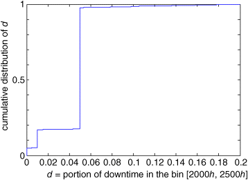
The CDF in Figure 9.4 has two main steps, which can be interpreted by considering the stochastic evolution of a population of identical components:
- The first step at
 is caused by the inspection of the components which have not failed before and are found in degradation state “Good.” These components are unavailable during the inspection which lasts for 5 h (= 1% of
  ).
). - The second step at
 is caused by CBM actions on the components which have not failed before and are found in degradation state “Medium” or “Bad.” These components require maintenance actions that last 25 h (= 5% of
  ).
).
Obviously, there are other contributions to ![]() , which are related to:
, which are related to:
- Replacement actions of the components failing in the previous bin, and reset into operation in the current bin; these components cause the smoothly increasing behavior of the CDF between
 and
and 
- Unavailability due to maintenance actions on components that have failed in the first bin (
 ) and are thus inspected between 2000 and 2500 h.
 - Unavailability due to failure of the components that have already experienced one or more failures in the previous bins.
Notice that the downtime in the bin is always smaller than 20% of its length; this is due to the fact that none of the components of the considered population has experienced more than one failure in the same bin, and the duration of a replacement action corresponds to 20% of the bin duration.
Figure 9.3(b) decomposes the average unavailability over a bin into its different constituents: unavailability due to the inspection of the component while it is in degradation state “Good”; unavailability due to preventive replacements if it is found in states “Medium” or “Bad” at inspection; and unavailability due to corrective maintenance actions that are performed upon failure.
By considering a population of components of the same type, a comparison of Figures 9.3(a) and (b) shows that the first increase of unavailability, at ![]() , is mainly due to the corrective maintenance actions that replace the components that failed within the time interval
, is mainly due to the corrective maintenance actions that replace the components that failed within the time interval ![]() . For this purpose, notice that the scale parameter of the Weibull distribution representing the transition from the degradation state “Good” to the degradation state “Medium” is equal to 1861 h, and since this quantity corresponds to the 63.21th percentile of the distribution of the transition time, it is expected that several components will have experienced the transition toward the state “Medium” and a small number of components will have even experienced a further transition toward the state “Bad.” The values of the failure rates associated with these latter states (
. For this purpose, notice that the scale parameter of the Weibull distribution representing the transition from the degradation state “Good” to the degradation state “Medium” is equal to 1861 h, and since this quantity corresponds to the 63.21th percentile of the distribution of the transition time, it is expected that several components will have experienced the transition toward the state “Medium” and a small number of components will have even experienced a further transition toward the state “Bad.” The values of the failure rates associated with these latter states (![]() and
and ![]() , respectively), which are larger than that associated with the “Good” state (
, respectively), which are larger than that associated with the “Good” state (![]() ), explain the increase in the number of components that fail in the interval
), explain the increase in the number of components that fail in the interval ![]() .
.
The average unavailability over the bins shown in Figure 9.3 reaches a maximum at ![]() , which refers to the bin
, which refers to the bin ![]() ; the sources of unavailability in this bin have been discussed above.
; the sources of unavailability in this bin have been discussed above.
In the successive bins, there is an increase in the number of components whose inspection and failure times are shifted with respect to the “crowd” (i.e., the large number of components experiencing the same behavior), and this leads to more smoothed peaks, due to replacement of components in the “Medium” degradation state, and larger average unavailability in the bins that follow these peaks, due to the replacement of components both failed and in the “Medium” degradation state. The unavailability due to replacement of components in the “Bad” state and inspections in the “Good” state remains small.
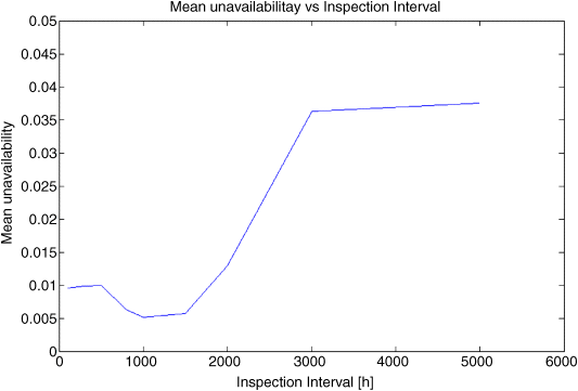
Figure 9.5 shows the average unavailability of the component in the mission time for different values of the inspection interval ![]() Initially, there is a decreasing behavior that reaches a minimum corresponding to
Initially, there is a decreasing behavior that reaches a minimum corresponding to ![]() ; for longer inspection times, the unavailability starts to increase rapidly. This is the result of two conflicting trends: on the one hand, more frequent inspections increase the probability of finding the component in degradation states “Medium” and “Bad”; this prevents the component from failing and thus avoids the corresponding long replacement time after failure. On the other hand, frequent replacements are ineffective, since component life is not completely exploited in this case. The minimum at
; for longer inspection times, the unavailability starts to increase rapidly. This is the result of two conflicting trends: on the one hand, more frequent inspections increase the probability of finding the component in degradation states “Medium” and “Bad”; this prevents the component from failing and thus avoids the corresponding long replacement time after failure. On the other hand, frequent replacements are ineffective, since component life is not completely exploited in this case. The minimum at ![]() represents the optimal balance between these two tendencies.
represents the optimal balance between these two tendencies.
Figure 9.5 Mean unavailability (EU) corresponding to different inspection intervals.
9.4.2 Application of the Hybrid Probabilistic–Theory of Evidence Uncertainty Propagation Method
We now consider the epistemic uncertainty on the parameters of the failure and degradation time distributions. The uncertainty propagation method described in Section 6.2.2 is applied to this level 2 uncertainty setting. The output of the model has been defined as a vector Z formed by ![]() elements: the first
elements: the first ![]() elements represent the portions of downtime in the corresponding bins, element
elements represent the portions of downtime in the corresponding bins, element ![]() represents the portion of downtime in the whole mission time, and the last bin represents the cost associated with the maintenance policy.
represents the portion of downtime in the whole mission time, and the last bin represents the cost associated with the maintenance policy.
As describe in Section 6.2.2, the uncertainty propagation method provides summary measures of the model output quantities. In this work, we focus on the mean values of the output quantities, that is, the average unavailability EU over the time bins that the mission time has been divided into, and the expected costs EC. Considering, for example, the average unavailability EU over the mission time, the method provides the belief and plausibility measures ![]() and
and ![]() for any interval of possible average unavailability values,
for any interval of possible average unavailability values, ![]() . The results will be illustrated considering intervals
. The results will be illustrated considering intervals ![]() with
with ![]() in
in ![]() , and the measures
, and the measures ![]() and
and ![]() will be referred to as belief and plausibility distributions.
will be referred to as belief and plausibility distributions.
The application of the uncertainty propagation method requires a fixed number of samples, ![]() , to be generated from the space of the uncertain parameters subject to epistemic uncertainty. Note that the larger the value of
, to be generated from the space of the uncertain parameters subject to epistemic uncertainty. Note that the larger the value of ![]() , the larger the number of output values, and, thus, the higher the precision in the identified pair of distributions
, the larger the number of output values, and, thus, the higher the precision in the identified pair of distributions ![]() . Therefore, setting
. Therefore, setting ![]() requires a trade-off between the precision of the distributions and the need to reduce the computational time. In this work,
requires a trade-off between the precision of the distributions and the need to reduce the computational time. In this work, ![]() has been set to 2000.
has been set to 2000.
9.5 Results
Figure 9.6 shows the obtained plausibility and belief distributions of the average unavailability over the different bins into which the mission time has been divided. In the first bins (i.e., from ![]() to
to ![]() ), the plausibility and belief distributions are very close to each other and reach 1 in correspondence to a value of the average unavailability very close (or even equal) to 0; this is due to the fact that the average bin unavailability tends to remain very small for any combination of the values of the epistemic uncertain parameters ranging in the intervals provided by the experts.
), the plausibility and belief distributions are very close to each other and reach 1 in correspondence to a value of the average unavailability very close (or even equal) to 0; this is due to the fact that the average bin unavailability tends to remain very small for any combination of the values of the epistemic uncertain parameters ranging in the intervals provided by the experts.
Figure 9.6 Plausibility and belief distributions of the mean values of the unavailability over time, obtained by the hybrid method (based on Baraldi, Compare, and Zio, 2013a).
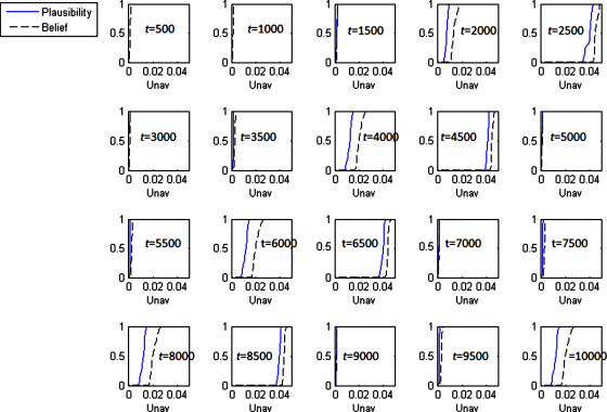
The situation is different at ![]() , when both plausibility and belief distributions are shifted toward higher values of the unavailability. This is due to an increase in the number of components that experience a failure in the bin
, when both plausibility and belief distributions are shifted toward higher values of the unavailability. This is due to an increase in the number of components that experience a failure in the bin ![]() , due to components' transitions toward the degradation states “Medium” and “Bad,” as explained above in the case without epistemic uncertainty (Section 9.4.1). Note also that the gap between the plausibility and belief distributions is quite large, when compared to those of the first bins. This is due to the fact that the behavior of the components is greatly influenced by the particular combination of the uncertain parameters. For example, considering that the scale parameter represents the 63rd percentile, a combination of the values
, due to components' transitions toward the degradation states “Medium” and “Bad,” as explained above in the case without epistemic uncertainty (Section 9.4.1). Note also that the gap between the plausibility and belief distributions is quite large, when compared to those of the first bins. This is due to the fact that the behavior of the components is greatly influenced by the particular combination of the uncertain parameters. For example, considering that the scale parameter represents the 63rd percentile, a combination of the values ![]() and
and ![]() leads to simulated histories in which it is very likely that the components experience a failure before
leads to simulated histories in which it is very likely that the components experience a failure before ![]() , with the consequent large unavailability; on the contrary, the combination
, with the consequent large unavailability; on the contrary, the combination ![]() and
and ![]() results in histories in which a failure in the bin
results in histories in which a failure in the bin ![]() rarely occurs.
rarely occurs.
In the next bin, at ![]() , the distributions are even more shifted toward the right part of the unavailability axis; this is in agreement with the behavior of the unavailability in the case with no uncertainty on the model parameters (Figure 9.3). In the successive bins (Figure 9.6), the plausibility and belief distributions follow the “cycle” of the first bins; for example, the curves relevant to the bin
, the distributions are even more shifted toward the right part of the unavailability axis; this is in agreement with the behavior of the unavailability in the case with no uncertainty on the model parameters (Figure 9.3). In the successive bins (Figure 9.6), the plausibility and belief distributions follow the “cycle” of the first bins; for example, the curves relevant to the bin ![]() are similar to the corresponding ones in the bin
are similar to the corresponding ones in the bin ![]() ; the differences between the plausibility distributions and the belief distributions pertaining to “similar” bins are due to an increase in the number of components that experience a life different from that of the “crowd,” as explained previously in Section 9.4.1.
; the differences between the plausibility distributions and the belief distributions pertaining to “similar” bins are due to an increase in the number of components that experience a life different from that of the “crowd,” as explained previously in Section 9.4.1.
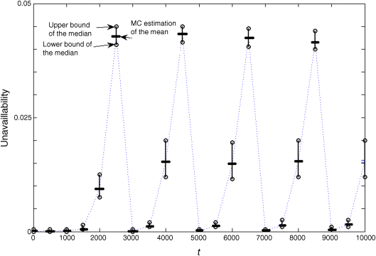
In an attempt to summarize the distributions in Figure 9.6, Figure 9.7 shows lower and upper bounds of the median of the average unavailability over the bins. The median represents the 50th percentile of the average unavailability in the bins. For comparison, the estimates of the average unavailability over the bins found in Section 9.4.2, where the epistemic uncertainty was not considered, are also provided in Figure 9.7.
Figure 9.7 Lower and upper bounds of the median of the average unavailability over the bins (based on Baraldi, Compare, and Zio, 2013a).
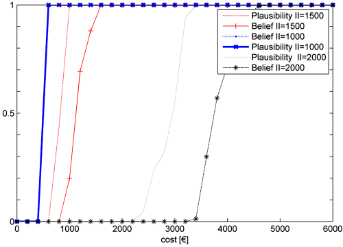
Figures 9.8 and 9.9 show the plausibility and belief distributions of the mean unavailability and cost over the mission time, respectively, corresponding to three different values of the ![]() , namely
, namely ![]() ,
, ![]() , and
, and ![]() . The small degree of uncertainty in the values of both unavailability and costs, when the component is inspected every 1000 h, derives from the fact that the “crowd” remains very compact. These figures clearly show that when the maintenance optimization problem involves epistemic uncertainty, identification of the best maintenance policy is not a trivial problem. For example, establishing whether the performance corresponding to
. The small degree of uncertainty in the values of both unavailability and costs, when the component is inspected every 1000 h, derives from the fact that the “crowd” remains very compact. These figures clearly show that when the maintenance optimization problem involves epistemic uncertainty, identification of the best maintenance policy is not a trivial problem. For example, establishing whether the performance corresponding to ![]() is better than that associated with
is better than that associated with ![]() is an open issue which needs to be addressed.
is an open issue which needs to be addressed.
Figure 9.8 Plausibility and belief distributions of the mean unavailability over the time horizon, for different values of the control variable II (based on Baraldi, Compare, and Zio, 2013a).
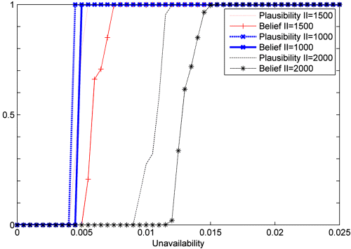
Figure 9.9 Plausibility and belief distributions of the expected cost EC over the time horizon, for different values of the control variable II (based on Baraldi, Compare, and Zio, 2013a).
A drawback of the method lies in the very large memory demands and computational times required, which result from the complexity of the algorithm. In fact, this requires that a number of MC trials are simulated to capture the aleatory uncertainty of the system for each of the ![]() samples from the
samples from the ![]() -dimensional space of the uncertain parameters (i.e.,
-dimensional space of the uncertain parameters (i.e., ![]() simulations). Furthermore, the mapping between the output and the
simulations). Furthermore, the mapping between the output and the ![]() -dimensional space (step 5 of the procedure in Section 5.2.2) is burdensome.
-dimensional space (step 5 of the procedure in Section 5.2.2) is burdensome.
Table 9.4 reports the computational times of the method for ![]() and
and ![]() combinations of values of the uncertain parameters.
combinations of values of the uncertain parameters.
Table 9.4 Computational time.
| Parameters | Values |
| Number of MC trials | 2000 |
| Number of combinations of uncertain parameters | 8000 |
| CPU time (Intel Core 2 duo, 3.17 GHz, 2GB RAM) | ≈30 h |
