
CHAPTER 9
Common Uses of Tools in Financial Modelling
Now that we know how to use many of the useful tools, functions, and features of Excel, let's take a look at actually using these tools to solve common problems, calculations, and situations encountered in financial models.
ESCALATION METHODS FOR MODELLING
There are several different ways of applying a growth, indexation, or escalation method over a period of time to a principal amount. We often need to be able to include escalation in our models for the purpose of forecasting sales growth year-over-year, for example, or increasing costs by an inflation amount. Calculating a growth amount might seem straightforward initially, but there are several different methods that can be used, and when applying growth rates in a model you need to be clear about which method you are using.
Whilst we can use functions to calculate future values based on set or varying growth rates, we'll first calculate them manually so that we understand the mechanics of the calculations, and then use the functions.
Using Absolute (Fixed) Growth Rate
Here we have compound growth over five years at a fixed interest rate. The capital grows each year by 5 percent. At the simplest level, our formula is ![]() The reason we are adding 1 (effectively 100 percent) to the growth rate (5 percent) is that we want the capital sum returned along with the accrued interest. Multiplying an amount by (1+growth) is a very common calculation technique when building financial models.
The reason we are adding 1 (effectively 100 percent) to the growth rate (5 percent) is that we want the capital sum returned along with the accrued interest. Multiplying an amount by (1+growth) is a very common calculation technique when building financial models.
Exercise: Fixed and Compounding You can create this example yourself in the following five steps, or you can find this template, along with the accompanying models to the rest of the screenshots in this book, at www.plumsolutions.com.au/book.
- Create the exercise as shown in Figure 9.1. The rate is fixed in a single cell (B4). Therefore, we need an absolute reference, namely $B$4. So, after the first year (in 2021), create the formula in cell C7:
 .
.

FIGURE 9.1 Fixed, Compounding Exercise
- Copy the formula in C7 to cells D7 through G7.
- This method grows the amount at a fixed rate, which compounds each year.
With most models, we normally want to show the amount that is forecast in each year, but if you want a shortcut formula that will show, in a single cell, how much we'll have at a fixed 5 percent growth after five years, we can use the Future Value (FV) function. Let's verify the amount you calculated for the year 2026 by using this function.
- Somewhere in a cell to the right of this table, enter Excel's FV function. Either type
 ( into the cell and follow the prompts, or select FV from the Insert Function dialog box. Because there are no periodic payments being made, we need to include the yearly rate, the period in years, and the present value (PV).
 - Prefix the function with a minus symbol to get a positive result. Your formula should be
 , and the totals using both methods should be the same. Your sheet should look something like Figure 9.2.

FIGURE 9.2 Completed Fixed, Compounding Exercise
Exercise: Fixed and Non-compounding Another variation on this escalation method is to still use a fixed growth rate, but not compound it. To do this, we will use an escalation index across the top. This may be more practical in some model designs but bear in mind that it yields different results. See Figure 9.3.

FIGURE 9.3 Fixed, Non-compounding Exercise
- In row 10, create your escalation index row using the formula
 in cell C10, and copying across.
 - Escalate in cell C14 by using the formula
 , and copying across.
This formula gives you a lower result in Year 5 than the exercise examining fixed and compounding interest because it is not compounding on the previous year. It simply adds a flat $5,015 × 5 percent each year, instead of adding the growth rate to the increased total.
Using Relative (Varying) Growth Rates
The next example returns the future value of an initial principal after applying a series of interest rates. While the rate was fixed in the example above, here it fluctuates from year to year. This is considered to be a superior model design, as it allows for fluctuation of growth rates. Even if the growth rate does not change from year to year, by building the model in this way, we are allowing for changes in the future. By using the aforementioned design with a single growth rate, we are restricted to having only a rate that does not change.
We'll no longer use absolute references for the interest rate but will allow both it and the value to change from year to year as we copy the formula across D22 through to G22. Cell C22's formula is ![]() , as previously, but this time the growth does not have an absolute reference applied to it. The formula is
, as previously, but this time the growth does not have an absolute reference applied to it. The formula is ![]() .
.
Exercise: Relative and Compounding
- Complete cell C22 in the exercise workbook as described above, then copy the formula to the right.
Let's try a shortcut function to get directly to the results without going through the annual calculations.
- To the right of the results, enter Excel's FVSCHEDULE function to verify the figure for 2026.
- Use the function FVSCHEDULE in your exercise spreadsheet.
Your sheet should look something like Figure 9.4.

FIGURE 9.4 Relative, Compounding Exercise and FVSCHEDULE Function
Exercise: Relative and Non-compounding In this next example, we are using another escalation index across the top. See Figure 9.5.
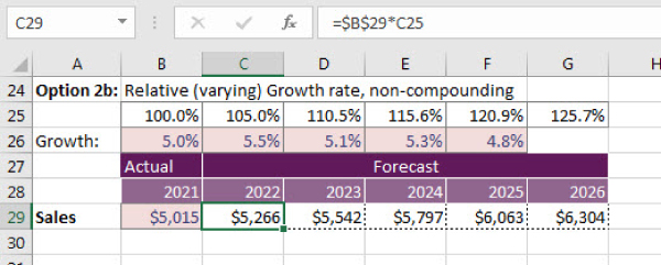
FIGURE 9.5 Relative, Non-compounding Exercise
- In row 25, create your escalation index row by using the formula
 in cell C25, and copying across.
 - Escalate in cell C29 by using the formula
 , and copying across.
This formula gives you a lower result in Year 5 than the fixed and compounding example, because it is not compounding on the previous year.
Using Exponential Operations on an Absolute (Fixed) Growth Rate
This exercise is similar to the first one, except that we will include the use of the caret symbol (![]() ) to perform exponential (to the power of) operations. For instance, 3 × 3 × 3 = 27. So does 33 and, in Excel's equivalent, 3
) to perform exponential (to the power of) operations. For instance, 3 × 3 × 3 = 27. So does 33 and, in Excel's equivalent, 3![]() 3.
3.
Exercise: Complex Escalation Figure 9.6 shows compound growth over a period at a fixed 5 percent per annum interest rate.

FIGURE 9.6 Complex Escalation
Our formula will allow for start and end dates to the period, in the form
Excel will perform the exponential operation before the multiplication, so the encompassing set of parentheses is not essential. The formula in C37 is therefore
Note that instead of using End year-Start year, you may also insert a helper row at the top to link to instead, which makes a slightly less complex formula. The next exercise shows how this can be done.
- Complete the formula for cell C37 and copy it across to achieve the results in the diagram below.
- The formula
 will verify the answer for the year 2026, as shown in cell I37 of Figure 9.6.
Practical Usage of Exponential Growth Rates
You will notice that we achieved the same result ($6,401) under the fixed, compounding exercise as we did under the relative and compounding exercise, but with a far less complex formula. Using exponential growth rates is useful when you need to compound the growth rate, but want each cell to operate independently.
If, for example, you have start dates and end dates that need to be included in a formula as well as compounding escalation, you will need to use exponential growth rates. In Figure 9.7, we will create a formula to evaluate the start date and end date, only inserting the cost in the relevant years and then compounding the inflation.

FIGURE 9.7 Completed Staff Calculation Using Exponential Growth Rates
This will require the IF and AND functions to be used in combination to establish whether the column heading year falls within an employee's start and end dates.
For instance, in English terms we will be checking that ![]() is true before writing inflation-escalated costs into the appropriate cell of column F. Otherwise we will write a zero.
is true before writing inflation-escalated costs into the appropriate cell of column F. Otherwise we will write a zero.
Use the term in years (row 5) to exponentially escalate the costs (in column C). For instance, if the year 2021 (F6) meets the IF test, F7 will equate to ![]() , which leaves it, in this case, unchanged.
, which leaves it, in this case, unchanged.
Your formula should be
and the sheet should look something like Figure 9.7.
UNDERSTANDING NOMINAL AND EFFECTIVE (REAL) RATES
From a financial modelling perspective, there are two interesting aspects of nominal and effective rates that we should be aware of.
- Escalation calculations. We need to consider whether an escalation, growth rate, or indexation amount includes the effect of inflation (i.e., whether it is real or effective) and what this actually means in real terms.
- Loan calculations. When comparing and calculating interest rates, the frequency of compounding can make a difference to the amount of interest actually paid. This can be calculated in Excel using the EFFECT and NOMINAL functions.
When including escalation or growth rates in a financial model, we sometimes need to consider whether the growth percentage is expressed as a nominal or real rate. Normally we express the growth percentage as a nominal rate, meaning that we don't take into consideration the effect of inflation or other factors that would impact the value of that rate. The real or effective rate will include the effect of other factors, such as inflation, to give you the real or adjusted value.
For example, if you earn a $100,000 salary, and after a year of working for the company your boss unexpectedly gives you a raise of 10 percent, you might think you're going to have an extra $10,000 in your pocket, right? Well, not exactly. Theoretically, in the 12 months since you began working for the company, your cost of living has increased and eroded the purchasing power of your salary. Therefore, if we assume that the consumer price index (CPI), or rate of inflation, is 3 percent, then your $100,000 is not buying you as much now as it did when you first started the job. To calculate the effective salary increase that you received, you'd need to deduct the inflation from the raise. Your nominal increase was 10 percent, but the real or effective raise was only 7 percent.
Normally, when modelling escalation amounts, we use the nominal rate and we know, when considering the calculations, that it does not take into account the purchasing power in the future. For example, in the exercise described in the previous section, we indexed the sales revenue at 5 percent, as shown below. It goes without saying that this 5 percent is a nominal amount. We know that the $6,401 received in Year 5 is not really $6,401 in today's terms, because inflation will have eroded its purchasing power. See Figure 9.2.
If we want to compare an investment in today's terms, we need to use the effective rate and to calculate this, we simply deduct the inflation amount—let's say 3 percent—from the growth rate, and hence our effective growth rate is 2 percent. As always, we need to be very explicit about the rates we have used. Note that expressing amounts in effective terms is not commonly used in financial models and, unless stated otherwise, the user would assume that a rate is nominal. Therefore, if you choose to use an effective rate, make sure that you state it clearly as an assumption, as shown in Figure 9.8.

FIGURE 9.8 Assumption Documentation in Growth Calculations
Adjusting Loan Rates with NOMINAL and EFFECT Functions
Calculating effective growth rates as outlined above is quite simple, and we certainly don't need a dedicated Excel function for this. There is another use for the nominal and effective concept in finance, and the calculation is far more complex. Nominal and real rates affect mortgage calculations, too. As discussed in “Loan Calculations” in Chapter 6, due to the effect of compounding, we actually pay a higher interest rate than is expressed in the nominal rate when quoted by the lender. Most loans are calculated and compounded daily, and therefore every single day we pay interest on the interest that was charged on the previous day.
The nominal rate is basically the simple interest rate for the complete period of the mortgage (i.e., the rate you are quoted when you take out the loan). The effective rate takes into account the compounding and will, therefore, be higher, depending on how frequently the loan is compounded.
The nominal and effective rates in Excel are related as follows:

where N is equal to the number of compounding intervals in the year.
As usual, Excel has made these calculations simple for us by offering two important predefined functions to convert nominal to effective rates, and effective to nominal. These are NOMINAL and EFFECT.
![]() . This function returns the annual nominal interest based on the effective rate and compounding intervals in the year. The syntax for this command is
. This function returns the annual nominal interest based on the effective rate and compounding intervals in the year. The syntax for this command is ![]() , where:
, where:
- Effective_Rate is the effective interest rate for the year.
- Compounding_Period is the total number of compounding intervals in the year.
![]() . This function returns the effective interest based on the annual nominal rate and compounding intervals in the year. The syntax for this command is
. This function returns the effective interest based on the annual nominal rate and compounding intervals in the year. The syntax for this command is ![]() , where:
, where:
- Nominal_Rate is the annual nominal interest rate for the year.
- Compounding_Period is the total number of compounding intervals in the year.
The next exercise shows how the effective rate can be calculated from the nominal rate.
Exercise: Comparing Two Nominal and Effective Interest Rate Offers Let's say you need to borrow some money, and you're offered two different interest rates from competing lenders.
- Lender A is offering a nominal rate of 7.9 percent, compounded daily.
- Lender B is advertising an effective rate of 8.2 percent, compounded monthly.
Which is the best deal? Here are four steps to arrive at the answer:
- Set up the inputs side by side, so that you can compare the effective rate, as shown in Figure 9.9.

FIGURE 9.9 Comparison of Interest Rates
- Calculate the effective rate of Offer A using the EFFECT function.
- Your formula in cell B4 should be
 .
.
The effective rate of Offer A is 8.2219 percent, which means that Offer B is, in fact, a lower effective rate.
Let's calculate the nominal rate of Offer B, for interest's sake.
- Your formula in cell C2 should be
 .
.
Let's see what effect the number of compounding periods has on the rate. If Lender A had compounded monthly instead of daily, would that have made a difference to the effective rate? It certainly would! Change the number of periods in cell B3 from 365 to 12, and we will see that this drops the effective rate to just slightly lower than that of Offer B. See Figure 9.10.

FIGURE 9.10 Comparison of Rates with Changed Compounding Periods
Although only a very simple calculation, this is a good example of how, by following financial modelling best practice and linking the formulas to the hardcoded input variables, we can easily perform sensitivity analysis on our numbers by changing the calculation assumptions.
CALCULATING A CUMULATIVE SUM (RUNNING TOTALS)
As always, we try to follow best practice when building financial models, and one of the important points of best practice is to ensure that formulas are as consistent as possible. Calculating a cumulative sum, or running totals, is common in financial modelling, and this is one such situation where ensuring consistent formulas can be tricky.
We need to calculate the cumulative number of customers in order to calculate the revenue, and Figure 9.11 shows one solution to the problem. It will achieve a correct total, but it necessitates using different formulas in adjacent cells.

FIGURE 9.11 Method 1: Cumulative Total Using Inconsistent Formulas
Sometimes this is the only solution (without creating an overly complicated formula) and, if necessary, you may simply need to resign yourself to the fact that consistent formulas are not possible. There is, however, a simple solution. Using the formula ![]() and then copying it across will achieve the same result with consistent formulas, as shown in Figure 9.12.
and then copying it across will achieve the same result with consistent formulas, as shown in Figure 9.12.

FIGURE 9.12 Method 2: Cumulative Totals Using a Consistent Formula
HOW TO CALCULATE A PAYBACK PERIOD
There is no dedicated formula in Excel (yet) for calculating a payback period. However, there are a couple of different ways of doing it manually. Demonstrated below are two methods, but this is by no means an exhaustive list. The first method is very simple, but not very accurate, and the second is quite long-winded, but more precise. You can find this template, along with the accompanying models to the rest of the screenshots in this book, at www.plumsolutions.com.au/book.
Simple Payback Calculation
In a business case summary, as shown in Figures 9.13 and 9.14, we can see that the payback period (the point at which the sum of our cash flows becomes positive) is between three and four years—at 2024. We can easily estimate this by highlighting the cash totals for each year and looking at the sum amount at the bottom right-hand corner of the page, as shown in Figure 9.13. However, we would like to create a cell that automatically calculates the payback year so that as inputs change due to scenario and sensitivity analysis, the payback year will always be shown in the model, based on the cash flow amounts.

FIGURE 9.13 Manually Calculating the Payback Year

FIGURE 9.14 Completed Simple Payback Calculation
- In row 14, create a formula that calculates the cumulative amount of cash. See “Calculating a Cumulative Sum” above for how to do this. Your formula should be
 .
. - In cell B16, insert a formula that will return the year in which the cumulative cash amount becomes positive. Remember that we want to look along the row and find the moment at which it becomes zero or greater. Your formula should be something like this:
 . For greater detail on how to use LOOKUP versus VLOOKUP or HLOOKUP, see “LOOKUP Functions” in Chapter 6.
 - Note that this formula is looking for a close match, which means that it will look along row 14 until it finds zero, and it will return the value before it passes zero. In this case, it will find the value under −1,677,907, as this is the last value before zero.
- This will give you the value 2023, but we actually want 2024, so simply add +1 to the end of the formula. Your formula should be
 .
. - Alternatively, you could add the cumulative calculation in row 2, and then use an HLOOKUP function to find the year at which the cumulative cash flow becomes positive. In this case, your formula in cell B16 would be
 . Having the cash flow showing above the years looks a little odd, so you'd probably hide it. I prefer the LOOKUP solution for this reason.
Note that this method is only a sample of several different tools and functions that could be used to calculate the payback period. For example, you could use a nested IF function instead, and an INDEX/MATCH combination. See Figure 9.14 for what your completed version could look like.
As the numbers for your business case change, so will your payback year. The result is only a rough estimate. For a more specific (albeit theoretical) payback date, we can use a more complex calculation, as shown in the following.
More Complex Payback Calculation
If you want to see exactly the year and month at which—theoretically—your project turns a profit, there is a more complex method. This way is also quite straightforward, but a little more time-consuming.
- On a new sheet, in column C, type in 1 Month 2 Months…1 Year and 1 Month, and so on, up to 10 years or so.
- In column A, insert the years that correspond to the months. In this case, the first year is 2021, so enter 2021 in cell A2. Copy this down, and change it to 2022 after 12 months. This can most easily be done by entering the formula A2+1 into cell A14 and copying it right down to the bottom.
- We are going to use column A as the criteria to pick up the cash in each year. In column B, enter a formula that will reference the profit and loss (P&L) page, and return the cash for that year, which should be divided by 12 to show the cash for each month. Your formula in cell B2 should be
 . This is (theoretically) how much cash the project has cost after one month of operation. We are assuming, in this formula, that the sheet containing your cash flow is called P&L.
 - Then make this a cumulative amount in column B, by changing the formula in Month 2 so that it adds to the previous total. Your formula in cell B2 should be
 . Copy this down the column.
Your sheet should look something like Figure 9.15.

FIGURE 9.15 Payback Period Workings
Unfortunately, the cumulative SUM calculation that was performed in the last exercise will not work in this instance, so we need to create an inconsistent formula. If this really bothers you, you could add a row and put a zero in cell B2 instead, so that the formulas are consistent.
- Continue this calculation right down the page until you reach Year 7 or 8, or as far as you want your payback calculations to work. Remember that if you're doing sensitivity and scenario analysis on this later, you don't want the formula to return an error if the calculations can't handle a larger value, so always go down a little bit further than you think you'll need.
- You can now perform a close-match VLOOKUP or LOOKUP, which will return the year and month at which the return becomes positive. This is the payback period.
- Enter the formula
 in the payback period cell on the P&L sheet. This will return the exact month and year that the project will hypothetically become profitable. See Figure 9.16. Of course, the close-match VLOOKUP will return the value preceding the value which is greater than zero. You may deem this to be close enough, or else move the months and years down by one row.

FIGURE 9.16 Completed Payback Calculation
WEIGHTED AVERAGE COST OF CAPITAL (WACC)
Before investing in a project or new venture, we need to evaluate whether the expected returns justify the risks. Many financial models are built for the purpose of new project evaluation, and the most commonly used tools that we use for evaluating the expected returns are NPV (net present value), IRR (internal rate of return), and payback period. How to calculate these measures is discussed in detail in “Financial Project Evaluation Functions” in Chapter 6.
However, in order to calculate the NPV, we need to know our cost of capital or our required rate of return for the project. You may also hear the cost of capital referred to as the discount rate or hurdle rate. The cost of capital is basically the opportunity cost of the funds invested, or, in other words, the rate of return that investors would expect to receive if they invested the money somewhere else, rather than in this particular project. In effect, by investing in the business, the investor is willing to forego the returns from other avenues. Therefore, cost of capital is the minimum required return for a project—the returns need to be greater than the cost of capital for the project to be accepted.
The importance of WACC is that it becomes a baseline to determine suitable investments for the success of the business. WACC is typically represented as a percentage, so any investment decisions taken by the company must aim to deliver returns greater than the WACC to make them worthwhile. For example, if the WACC of a company is 15 percent, then most of the investments that the company makes must be with the goal of generating returns greater than 15 percent. WACC is not just calculated for the entire company or business. It can also be calculated for individual projects to determine if it is worthwhile for the company to pursue the project.
Company capital is sourced from many avenues and is targeted for various areas of business growth and sustenance. Typically, the two major sources of capital are debt and equity. Both these tools are distinctly different, have different costs, and hence need to be considered differently in our calculations. As a result, not all capital carries the same weight, which is why we sometimes need to calculate the WACC in order to work out how much our capital is worth. Sometimes, when calculating the NPV of a project, a modeller may simply use a nominated cost of capital (we used a rate of 12 percent in the section “Net Present Value” in Chapter 6), but to evaluate a project more accurately, we can calculate which WACC will give us the exact cost of capital for that company. Note that the WACC will be completely different for each company, depending on its individual mix of equity and debt.
How to Calculate the WACC
The WACC is the average return on capital weighted proportionally based on category. Typically, a company sources its capital from stocks (common and preferred), bonds, and long-term debts. Each category of capital is invested in different avenues to help the business sustain and grow. WACC represents the average cost of capital, with proportional contributions from the various sources.
WACC can be calculated using the given formula:

where:
- Debt = total capital raised from debts.
- Equity = total capital raised from equity. Note that if the company has common and preferred shares, then the two need to be weighted and factored accordingly.
- Cost of debt = the cost of raising the debt. If taken as bank loans, then it is the interest that needs to be paid to the banks.
- Cost of equity = the return that the shareholders or investors expect from their holding in the company. Common ways of calculating this are the capital asset pricing model (CAPM) or Gordon's growth model.
- Tax rate = the prevalent corporate tax rate.
Exercise: Calculating the WACC in Excel While the formula looks very complex, once the concepts are clear, WACC can be calculated relatively easily in Excel. Let's do an exercise where we need to manually calculate the WACC.
Let's say you have the following inputs:
- Debt is $6,023,000, for which you are paying 8.5 percent.
- Equity is $4,421,000, for which you expect a return of 15 percent.
- Tax is 30 percent.
- Set up your sheet as shown in Figure 9.17.

FIGURE 9.17 WACC Calculation Layout
- In row 4, calculate the cost of debt and equity before tax.
- Your formula in cell B4 should be
 . Copy it across to cell C4.
 - In row 6, remove the tax from the debt amount.
- Your formula in cell B6 should be
 . Copy it across to cell C6. Although there is no tax applicable to the equity amount, we'll still copy the formula across to maintain consistency of formulas (hence following best practice).
 - Add together the value of debt and equity in cell D2, and cost after tax in cell D6.
- Now calculate the WACC, which will be the cost after tax of debt and equity as a proportion of the total.
- Your formula in cell D7 should be
 , and your worksheet should look something like Figure 9.18.

FIGURE 9.18 WACC Completed Calculation
Hence, the weighted average cost of capital for this company is 9.78 percent. This means that when this company is evaluating new opportunities, the minimum required rate of return would be 9.78 percent, as this is what its capital is currently costing it. When calculating the NPV for a new project, this would be the input for the discount rate in the NPV function. Theoretically, the NPV at this discount rate must be greater than zero, and the IRR of a series of cash flows needs to be higher than this amount in order for a project to be accepted.
BUILDING A TIERING TABLE
Calculating an amount based on tiering tables is a pretty complex formula, and is commonly used in pricing models. There are two types of tiering tables (also called volume breaks, block, or stepped pricing). The simplest version calculates the entire amount at the tier. The more complex table, like the tax tiers, is progressive such that the first number of units is calculated at the first tier and the next number of units at the next tier, and so forth.
For example, in a tax table where an income of $8,000 would be taxed at zero for the first $6,000 and then the next $2,000 is taxed at 15 percent, you would only pay $300 (15 percent of $2,000), not 15 percent on the whole amount.
Flat Tiering Structure
Let's say, for example, you have the pricing structure shown in the pricing table in Figure 9.19. If the customer purchases 5 items, each item costs $15, but if the order is for between 6 and 50 items, they are priced at $12 each, and so on.

FIGURE 9.19 Completed Flat-Tiered Pricing Calculation
We'd like to calculate how much a customer would be charged at different volumes.
A horribly long and complicated IF statement will do the trick:
Alternatively, an IFS statement is somewhat easier to build, but not much easier to follow:
For an example of how to build these formulas, refer to the section “Nesting Multiple IF Statements” in Chapter 5, but there is a much simpler way to build a tiering table using a close-match VLOOKUP or LOOKUP.
- In cell B3, calculate the per unit price using a close-match VLOOKUP. Your formula should be
 .
.
- Multiply the unit price by the number of units and add them up. Your total should be $7,564, and your sheet should look something like Figure 9.19.
Progressive Tiering Structure
If the tiering calculation is not as straightforward as that in Figure 9.19, we may need to calculate under a progressive tiered structure. A good example of this is the way that the Australian tax calculations work, as shown in Figure 9.20. This formula calculation is not for the faint-hearted, so unless you specifically need to calculate a progressive tiering table, feel free to skip this section. You can find this template, along with the accompanying models to the rest of the screenshots in this book, at www.plumsolutions.com.au/book.

FIGURE 9.20 Tiered Personal Australian Tax Calculation Example
The first person's salary is $123,120, which means that this person is in the $80,000 to $180,000 tax bracket. However, we can't do a flat tiering calculation on this because the first $18,200 is tax-free, the next bracket is only taxed at a rate of 19 percent, and so on. The formula in column I takes care of the calculations below the threshold. Note that the tiers begin with one cent (e.g., $18,200.01).
You'll need to split your calculation into several parts, as shown in the diagram. First, work out the lowest tier, and then calculate the difference between the salary and the tier (in this case $80,000). Then the remainder should be calculated at the marginal tax rate.
- Start by using a close-match VLOOKUP to pick up column I (the amount payable up to the threshold). Your formula should be
 .
. - Next, we need to work out the amount of the total salary that is above the lowest tier (in this example, $123,130 − $80,000 = $43,130). To do this, we'll do another close-match VLOOKUP returning the first column and subtract this from the salary amount. In a separate cell, your formula should be
 . Your answer should be $43,130.
 - Next, we need to find out how much to multiply the $43,130 by (i.e., the highest tax tier). To do this, create a VLOOKUP returning the third column. Your formula should be
 . Your answer should be 37 percent.
 - Now, put all three formulas together:

The good news is that if you've used cell referencing correctly, you can simply copy the formula down. See Figure 9.21.

FIGURE 9.21 Completed Progressive Tiered Calculation
MODELLING DEPRECIATION METHODS
How we treat capital expenditure, its effect on cash flow, and the subsequent depreciation is an important part of financial modelling—especially if your model includes a P&L statement, cash flow, and balance sheet. Capital expenditure is calculated and recorded in several different places:
- In the cash flow in the period in which it was purchased.
- On the balance sheet as a fixed asset.
- On the P&L statement as depreciation over the useful life of the asset.
In this section, we will focus on translating a purchase of a fixed asset into a depreciation charge to be shown on the P&L.
Why Depreciate?
The definition of a fixed asset is an asset that is used in production, or that supports business activities in some other way. Common examples are machinery, vehicles, and equipment such as computer hardware. Fixed assets, by definition, have an expected useful life of more than 12 months, and the cost of these assets must, therefore, be written off as an expense over the period in which they are used. Depreciation is the charge calculated to write off these assets over their expected useful lives.
In the examples that follow, in Year 1 we purchase a piece of machinery for $200,000 that has a useful life of five years (i.e., it will be generating income for the next five years), as shown in Table 9.1.
TABLE 9.1 Depreciation for a $200,000 Piece of Machinery
| Year 1 | Year 2 | Year 3 | Year 4 | Year 5 | |
| Sales | $150,000 | $160,000 | $170,000 | $180,000 | $190,000 |
| Machinery | ($200,000) | ||||
| Net Income | ($50,000) | $160,000 | $170,000 | $180,000 | $190,000 |
| Year 1 | Year 2 | Year 3 | Year 4 | Year 5 | |
| Sales | $150,000 | $160,000 | $170,000 | $180,000 | $190,000 |
|
Machinery Depreciation |
($40,000) | ($40,000) | ($40,000) | ($40,000) | ($40,000) |
| Net Income | $110,000 | $120,000 | $130,000 | $140,000 | $150,000 |
Instead of expensing the whole cost in Year 1, we should spread the cost of it over the five years, as this is a much more accurate method of showing the profitability in each year.
Adjusting depreciation is an attractive way for companies to increase expenses and lower taxable earnings, and for this reason, the regulatory legislation around which method of depreciation can be used is strictly monitored by the tax office. Bear in mind that finance and accounting rules differ between countries. Financial modellers do not need to be accountants, but they do need to ensure that accounting, tax, and finance rules are applied correctly if the calculation method is material to the model.
Depreciation Methods
In the example above, we have used the most common form of depreciation, which is the straight-line method. Under this method, the cost is equally spread over the number of years it is in use. However, there are several more complex depreciation methods also in use. It can be calculated either by using both a fixed rate and a fixed depreciable base value, or by varying one or both of these variables. For this reason, the depreciation charge each year as calculated by the different methods will not be the same. Figure 9.22 illustrates the charges each year.

FIGURE 9.22 Comparison of Different Depreciation Methods
The exercise below will show step by step how to calculate depreciation using the different methods, and by doing this, we'll see how very different each of the methods is. This is not an exhaustive list of depreciation methods; rather it's an overview of the most common forms of depreciation calculations used in financial modelling.
Straight-Line Method (=SLN Function) Straight-line depreciation (also called prime cost method) is the simplest and most used technique that calculates depreciation at a fixed rate over the expected useful life of an asset. We estimate the residual value (salvage or scrap value) of the asset at the end of its useful life and will expense a portion of the original cost in equal increments over that period. The salvage value is an estimate of the value of the asset at the time it will be sold or disposed of, but often it is zero. If the asset is expected to have a salvage value at the end of its useful life, we need to take the salvage cost away from the base before depreciating it. The formula for calculating depreciation is, therefore:
For example, we purchase an asset for $50,000, its useful life is 10 years, and we think we can sell it for $5,000 at the end of its useful life. We'd simply calculate the amount to be depreciated, which is the cost of the asset minus the residual value ![]() and divide it by 10, so the depreciation amount on the P&L would be $4,500 per year for 10 years.
and divide it by 10, so the depreciation amount on the P&L would be $4,500 per year for 10 years.
It's pretty easy to work this method of depreciation by using this sort of formula: ![]() , or you could use the SLN formula:
, or you could use the SLN formula: ![]() , which will deliver the same result.
, which will deliver the same result.
Calculating depreciation using the straight-line method is by far the most common method of calculating depreciation in financial modelling.
In order to demonstrate the comparison of the different methods, let's take a look at Figure 9.23, which shows an asset that has a purchase price of $50,000, a salvage value of $5,000, and a useful life of 10 years.

FIGURE 9.23 Asset Depreciation Example
To prepare a depreciation schedule for this asset in Excel using the straight-line method, the following steps are followed:
- Using an SLN formula, calculate the depreciation per year in row 11 columns B to K.
- Your formula in B11 should be
 . This formula requires cost value, salvage value, and life in years.
 - Once the absolute value signs have been added, the formula in B11 can be copied across into columns C to K. Using the straight-line method, the depreciation charge for each year is the same.
- The amount in each year should be $4,500. After completing the table, check that the total is equal to the cost less salvage value.
Declining Balance Value Methods
These methods are also called the reducing balance, diminishing value, or accelerated methods. You could argue that assets are more useful when they are new, and therefore depreciate more quickly in the first few years of acquisition. Therefore, some companies use depreciation methods that provide for a higher depreciation charge in the first year of an asset's life and gradually decrease charges in subsequent years. These are called accelerated depreciation methods.
Fixed Declining Balance Method (=DB Function) The fixed declining balance method calculates depreciation at a fixed rate. This rate is calculated by the formula
but it's much easier using the ![]() Excel function. The depreciation charge for each period is not the same, as the depreciation rate for a period is applied to the net book value at the beginning of that period, and not to the original cost. With this method, the starting net book value is the cost price, so depreciation is applied to cost and not the value of cost less salvage. This is because using this method, the net book value can never reach zero.
Excel function. The depreciation charge for each period is not the same, as the depreciation rate for a period is applied to the net book value at the beginning of that period, and not to the original cost. With this method, the starting net book value is the cost price, so depreciation is applied to cost and not the value of cost less salvage. This is because using this method, the net book value can never reach zero.
Instead of treating each year the same, the fixed declining method depreciates more quickly in early years and more slowly in later years. The book value of the asset at the beginning of the period is multiplied by a fixed rate (e.g., in Year 1, 10 percent of $45,000 is $4,500 of depreciation). In Year 2, the same 10 percent is multiplied by the remaining $40,500 of book value, which then gives a depreciation value of $4,050.
The most difficult part in the fixed declining method is to figure out the correct percentage to use for each year, which is done with a rather complicated algebraic formula. If you use the predefined DB function in Excel, however, you don't need to be concerned with the calculations. Bear in mind, however, that when Excel calculates the rate, it rounds to three decimal places, and this does cause the calculation to be off by a few dollars at the end of the useful life.
Therefore, unlike the straight-line method, you pretty much have to use the Excel formula. Using the example above, your fixed declining formula for Year 1 would look like this: ![]() .
.
Applied to the example above, to prepare a depreciation schedule for a particular asset in Excel using the fixed declining balance method, the following steps are followed:
- Using a DB formula, calculate the depreciation per year in row 12, columns B to K.
- Your formula in B12 should be
 . This formula requires cost value, salvage value, life in years, and period for which depreciation is being calculated.
 - Note that the additional requirement of a specified period is a result of the depreciation calculated each year being unique to that particular year or period. For this formula to return an accurate result, both life and period must be entered using the same unit (e.g., years).
- Once the absolute value signs have been added, the formula in B12 can be copied into columns C to K.
- If you create a total in L12, this will not be exactly equal to cost less salvage, as was the case for the straight-line method. This is a result of the fixed declining balance method producing a hyperbolic function and not a linear function and, therefore, never allowing the net book value to be zero.
- Once the table has been completed, check that the total calculated in L12 is not more than cost less salvage. If this is the case, a manual adjustment to the last period's depreciation charge will be required.
Your worksheet should look something like Figure 9.24.

FIGURE 9.24 Calculating Fixed Declining Depreciation
Double Declining Balance Method (=DDB Function) The double declining balance method also calculates depreciation at a fixed rate. This rate per annum is calculated as
Again, the Excel function (=DDB) makes this calculation a lot easier. As with the fixed declining balance method, the depreciation charge for each period is not the same. This is a result of the depreciation rate being applied to the net book value at the beginning of each period, and not to the original cost. Here, too, the starting net book value is the cost price and not cost less salvage. This method is quite similar to the fixed declining method shown above, except that the first year's depreciation uses double the percentage of the straight-line method. For each additional year of the asset's life, the opening book value is multiplied by the same percentage. When the amount calculated by the double declining method is less than what it would have been using the straight-line method, then the straight-line method is used.
In the example above, using the double declining balance method, the depreciation rate would be 20 percent in the first year instead of 10 percent using the straight-line method. This amount then reduces until it is less than $5,000, and then it switches to the straight-line method.
Using the DDB function, the formula would look like this:
To prepare a depreciation schedule for a particular asset on Excel using the double declining balance method, the following steps are followed:
- Using a DDB formula, calculate the depreciation per year in row 13, columns B to K.
- Your formula in B13 should be
 . This formula requires cost value, salvage value, life in years, and period for which depreciation is being calculated.
 - Once the absolute value signs have been added, the formula in B13 can be copied into columns C to K.
- Once again, the total in L13 will not be exactly equal to cost less salvage, as was the case for the straight-line method. This is a result of the double declining balance method also producing a hyperbolic and not a linear function.
- Once the table has been completed, check that the total calculated in L13 is not more than cost less salvage. If it is, a manual adjustment to the last period's depreciation charge will be required.
Your worksheet should look something like Figure 9.25.

FIGURE 9.25 Calculating Double Declining Depreciation
Sum of the Years' Digits Method (=SYD Function) Unlike the previous three methods of calculating depreciation, the SYD method calculates depreciation at varying rates for each period. As with the straight-line method, however, it uses a constant depreciable base, being cost less salvage value. The sum of the years' digits is calculated as
where n is equal to the useful life in years.
Depreciation for each period is then calculated as

The sum of the years' digits is a depreciation method that results in a more accelerated write-off than the straight-line method, but less than the declining balance method. Under this method, annual depreciation is determined by multiplying the depreciable cost by a schedule of fractions.
Use the Excel formula ![]() . To prepare a depreciation schedule for a particular asset on Excel using the sum of the years' digits method, the following steps are followed:
. To prepare a depreciation schedule for a particular asset on Excel using the sum of the years' digits method, the following steps are followed:
- Using an SYD formula, calculate the depreciation per year in row 14, columns B to K.
- Your formula in B14 should be
 . As with the previous two methods, this formula requires cost value, salvage value, life in years, and period for which depreciation is being calculated.
 - Once again, the additional requirement of a specified period is a result of the depreciation calculated each year being unique to that particular year or period. Unlike with the two previous methods, however, the difference in yearly depreciation charges is a result of a change in rate and not a change in the depreciable base.
- Once the absolute value signs have been added, the formula in B14 can be copied into columns C to K.
- Check that the total in L14 is, as with the straight-line method, exactly equal to cost less salvage value. Despite using varying rates, this method also produces a linear function.
Your worksheet should look something like Figure 9.26.

FIGURE 9.26 Calculating Sum of the Years' Digits Depreciation
Of course, there are many other methods of depreciation, most of which also have an Excel function, to make what would otherwise be an extremely complicated calculation much easier. Don't completely rely on the function, however! As always, sense-check the results and double-check the timing of the purchase date and the period at which the asset is deemed to be fully depreciated.
Calculating Depreciation at the End of Useful Life
When building a model to depreciate assets using the straight-line method, whether calculating it longhand or using the SLN function, it is possible to continue to calculate depreciation on an asset that has already been fully depreciated past its useful life. This results in an ever-increasing negative net book value, which is impossible and can be the cause of an error in the model.
In order to prevent depreciation from being calculated once the asset has reached the end of its useful life, the Excel depreciation formula needs to be amended.
Let's say you have a list of capital items in a database, as shown in Figure 9.27. You can find this blank template, along with the completed version and other accompanying models to the rest of the screenshots in this book, at www.plumsolutions.com.au/book.

FIGURE 9.27 Completed Depreciation Calculation on Fixed Assets
The first item on the capital expenditure register is for some IT equipment that was purchased in June 2018. The useful life is three years, which means that it will be fully depreciated in June 2021, and therefore if we create a forecast model for 2021, we need to ensure that the depreciation does not continue past the end of its useful life, and we need to create a formula to do this.
This will be a rather long formula, but we'll use a simple building block methodology where we create a simple formula, test it, and check it before adding to it. We then test and check it again, before adding to it. In this way, we minimise errors by making sure the formula syntax is correct.
Begin by calculating the depreciation for January 2021 for the asset in cell G4, using the straight-line depreciation method. Remember it's for a month, not a year. Your formula should look like this:
Test this by copying across and down the page to make sure that the cell referencing is correct.
- Once we've got this right, we need to consider the spend date. In some instances, the spend date for the item has not yet elapsed, so we need to evaluate whether this date has passed or not, and only allow the depreciation to show if the date has passed. We can achieve this by inserting an IF statement around the SLN function like this:
 . Test this by copying across and down the page to make sure that the cell referencing is correct.
 - Now we need to consider the end of useful life date. We could do this all in one formula, but it will make our calculations easier to follow if we insert this as a date within the model. In cell F4, calculate the date at which the item will be fully depreciated. We can do this using the formula
 . However, note that it gives you a value of 29th June 2021, because 2020 is a leap year. You can get around this by using the EOMONTH or DATE functions or by using 365.25 instead of 365—or you can simply leave it as it is (it won't make a lot of difference to our calculations). Copy the formula down column F.
 - Next, we need to add in the end of useful life date to our formula in cell G4. The best way to do this is by nesting an AND function with the IF. Your formula should look like this:
 .
. - Copy the formula across and down, and test to see if it is working correctly. The depreciation of the IT equipment should stop in July 2021.
Your worksheet should look something like Figure 9.27.
BREAK-EVEN ANALYSIS
Including break-even analysis in a financial model is very useful for budgeting purposes and especially for any business that is starting or expanding its operations. Break-even analysis is a very effective tool to determine profitability and give you a snapshot of the sales volume target that is required to start making a profit. For a new startup venture, this analysis is very effective in projecting sales targets. For established companies that are looking to launch new products and services, this analysis is invaluable in developing the pricing strategy.
There are several different ways to carry out the break-even analysis, depending on the perspective you want to look at. If you keep your pricing fixed, you can determine the units you need to produce and sell to break even (zero profit and zero loss). On the other hand, if your market position allows you to change the pricing, then you can determine the optimal pricing strategy to make your department or business break even within the stipulated target sales.
Let's take an in-depth look at some of the different methods of calculations for break-even analysis. It is also very helpful to show break-even points graphically, so we will also include some line charts when calculating the break-even points in our model in this section.
Calculating the Break-Even Point
The break-even point is dependent on the total cost of production, the price of units, and the number of units. In its most simplified form, the break-even point is achieved when:
The cost of production is never completely fixed. There is a variable component to it, which is related to the total units produced. This component includes everything from the price of raw materials to labour costs and additional overheads. Thus, the total cost of production is the sum of the fixed costs and the variable costs:
By varying the total number of units and/or the selling price of each unit, you can calculate the break-even point for your business. Figure 9.28 shows an example of the example of the profitability of the product at different volumes: 0, 1000, 2000, 3000 and 4000 units of sales. We can see how the variable costs change, while the fixed costs do not.

FIGURE 9.28 Break-Even Calculations
Example Using Excel Let's look at an example of how to calculate the break-even point for a new product. Let's say you want to start producing custom-made bird cages. You have determined that your fixed and variable costs for the first year are as follows:
- Fixed costs $250,275 (this includes rent, machinery, electricity, etc.).
- Raw materials of $5 per cage.
- Labour of $25 per cage.
- Overhead of $10 per cage.
Using the layout in Figure 9.28, calculate the net profit at each level of production. Ensure you use consistent formulas. At what level of production does the business begin to make a profit? The answer follows in the numbered list.
- Fixed costs will remain at $250,275 regardless of the production level. The formula in cell F5 should be
 . Copy it across.
 - Variable costs will fluctuate depending on the volume produced. The formula in cell F6 should be
 . Copy it across.
 - Add together the fixed and variable costs in row 7.
- Calculate the total revenue in row 8. The formula in cell F8 should be
 . Copy it across.
 - Now calculate the net profit at the various production volumes in row 9.
- The formula in cell F9 should be
 . Copy it across.
Your worksheet should look something like Figure 9.28. The completed version of this exercise can be found, along with the accompanying models to the rest of the screenshots in this book, at www.plumsolutions.com.au/book.
We can see that somewhere between 2,000 and 3,000 cages is when the revenue begins to cover our costs.
Charting the Break-Even Point
It is also interesting to look at the numbers graphically, and we can create a line chart that shows the point at which the revenue from the business becomes greater than the cost. See Figure 9.29.

FIGURE 9.29 Chart Showing Break-Even Point
For detailed instructions on how to create this chart, see the supplementary material available at www.plumsolutions.com.au/book.
We can see that the break-even point is roughly just under 3,000 units by looking at the chart, but this can be a pretty laborious task when done manually, and it is also not very accurate. We can calculate it exactly, however, using two methods in Excel:
- A formula calculation.
- A goal seek.
Calculating Break-Even Using a Formula Using a formula is the fastest way of calculating the break-even point. It can be calculated using the following formula:
Price minus variable costs gives you the gross profit or contribution of each unit. We can then divide the fixed costs by the contribution to see how many units need to be sold to cover the fixed costs. See Figure 9.30.

FIGURE 9.30 Break-Even Number of Units Using a Formula
In our model, we can calculate the break-even point by using this formula:
The Excel formula in our model to calculate this is ![]() .
.
Break-Even Analysis Using Goal Seek
Another way to perform break-even analysis is to use the goal seek tool. For a refresher on how to use this tool, refer to the “Goal Seeking” section in Chapter 8. While this method takes a little longer to set up and run than using a formula as described above, it is more flexible and allows more options for changing inputs.
Using our Bob's Bird Cages example, we need to set up the sheet as a simple P&L calculation, as shown in Figure 9.31.

FIGURE 9.31 Using Goal Seek to Calculate Break-Even Point
The number of cages produced is the unknown variable, and we have entered a value of 2,500 in cell C11 as a placeholder in the meantime (which we can see generates a loss). This is the variable that will change when we perform the goal seek. Remember that to perform a goal seek we need a formula and a hardcoded number that drives that formula. The formula will be the profit/loss amount in cell C16, and the hardcoded number is the number of cages in cell C11. Make sure that all of the formulas in cells C13 to C16 contain formulas; otherwise, the goal seek won't work.
So, to perform break-even analysis, we need to set the net profit/loss value to zero by changing the number of cages produced. See Figure 9.31.
When you click OK, Excel calculates the exact break-even point and edits the cell value accordingly, as shown in Figure 9.32.

FIGURE 9.32 Completed Break-Even Goal Seek
We can see that we end up with a value of 2944.41176470588. You might like to round it to the nearest unit, which will show a small profit or loss, which might be confusing. Alternatively, change the formatting so that the decimal places don't show.
If you have the power to manipulate the unit pricing, then you can change the price points to reach break even at the sale of a fixed number of units, and even set profit targets using the goal seek function. Let's say you don't think you can sell more than 2,500 units. What would you need to set your price to in order to make a profit of $50,000 if the maximum you will sell is 2,500? Because of the way we have set up this model, this is relatively easy to calculate. See Figure 9.33.

FIGURE 9.33 Break-Even Goal Seek with Changed Inputs
If we want to make a profit of $50,000, we'd need to sell 2,500 cages at $160 each.
Whilst the goal seek method takes a little longer to run and set up, it's a great way to run different scenarios and test changes in inputs when performing break-even analysis. If this is something you want to run repeatedly, consider setting up a macro button to run the goal seek. (See the section on Macros in Chapter 8 for more information on how to do this.)
SUMMARY
In the first part of this book, we covered the tools, functions, and techniques that financial modellers need to know. In this chapter, we focused on the use of these tools in a financial modelling context. If you are pursuing a career as a financial modeller, you will almost certainly have to calculate escalation at some point, and it is quite likely that you will find yourself needing to use tiering tables, calculate depreciation, or perform break-even analysis.