5.5. Modeling Relationships

For a traditional confirmatory analysis, Jane needs to use an analysis method that permits hypothesis testing. She could use logistic regression, with Defect (<=5%) as her nominal response. However, Jane feels that the partition analysis provided a good examination of this response and, besides, the continuous variable % Price Increase should be more informative. For this reason, she decides to model % Price Increase as a function of the Xs using Fit Model.

But which Xs should she include? And what about interactions, which the partition analysis clearly indicated were of importance? Fit Model fits a multiple linear regression. Jane realizes that for a regression model, nominal variables with too many values can cause issues relative to estimating model coefficients. So she needs to be selective relative to which nominal variables to include. In particular, she sees no reason to include Customer ID or Sales Rep, as these variables would not easily help her address root causes even if they were significant.

Now Region, thinks Jane, is an interesting variable. There could well be interactions between Region and the other Xs, but she does not see how these would be helpful in addressing root causes. The sales representatives need to be able to sell in all regions. She decides to include Region in the model to verify whether there is a Region effect (her exploratory work has suggested that there is not), but not to include any interactions with Region.

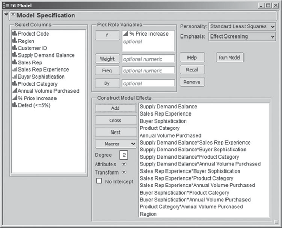
Jane builds her model as follows. She selects Fit Model from the Analyze menu. She enters % Price Increase as Y, and then, in the Select Columns list, selects the five variables highlighted in Exhibit 5.40. Then, to include two-way interactions involving these five variables, she clicks on the arrow next to Macro and selects Factorial to Degree from the drop-down menu. By default, this enters the effects for a model that contains main effects and all two-way interactions.

Figure 5.40. Fit Model Dialog

Now, she selects Region from the Select Columns list and clicks Add to add it to the Constructed Model Effects lists. The final Fit Model dialog is shown in Exhibit 5.41. From the menu obtained by clicking the red triangle next to Model Specification, Jane chooses Save to Data Table, which saves the script with the name Model. She renames it Model—% Price Increase.

Figure 5.41. Populated Fit Model Dialog

Jane clicks Run Model, and the report in Exhibit 5.42 appears. Jane examines the Actual by Predicted plot, noticing that the data seem randomly spread about the solid line that describes the model. There are no apparent patterns or outliers. (We will not delve into the details of residual analysis or, more generally, multiple regression at this time; there are many good texts that cover this topic.) So Jane concludes that the model appears to provide a reasonable fit to the data.

The Analysis of Variance table shows a Prob > F value that is less than .0001. This indicates that the model successfully explains variability in the response.

When the report window first opens, the Parameter Estimates panel is open. Jane realizes that this table gives estimates of the model parameters and provides a significance test for each. However, four of her predictors are nominal. Two of these have three levels and one has four, so the model parameterization involves indicator variables associated with these levels and their associated two-way interactions. She clicks the disclosure icon to close this panel.

To determine which effects are significant, Jane proceeds to examine the Effect Tests. She uses the usual 0.05 cut-off value to determine which effects are significant. She looks through the list of Prob > F values, identifying those effects where Prob > F is less than 0.05. She notes that JMP conveniently places asterisks next to these Prob > F values. The significant effects are:

Figure 5.42. Fit Least Squares Report

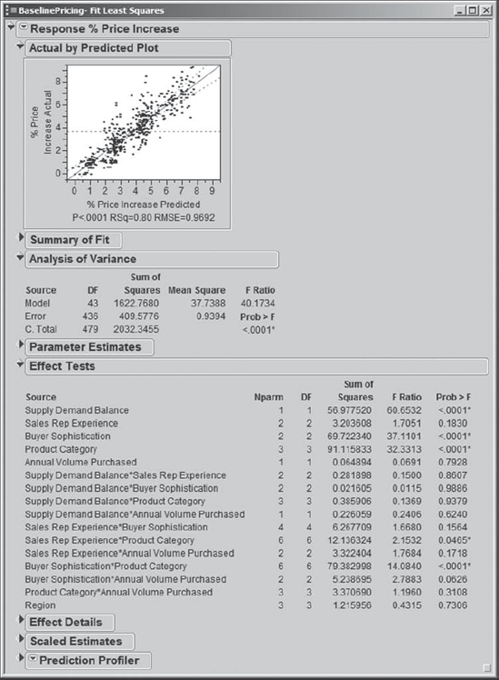
• Supply Demand Balance

• Buyer Sophistication

• Product Category

• Sales Rep Experience*Product Category

• Buyer Sophistication*Product Category

What is very interesting is that Sales Rep Experience has appeared in the list. On its own, it is not significant, but it is influential through its interaction with Product Category. This is an insight that did not appear in the exploratory analyses that Jane had conducted. In fact, Jane's exploratory results led her to believe that Sales Rep Experience did not have an impact on defective sales negotiations. But you need to keep in mind that Jane's multivariate exploratory technique, the partition analysis, used a nominal version of the response. Nominal variables tend to carry less information than do their continuous counterparts. Also, partition and multiple linear regression are very different modeling techniques. Perhaps these two observations offer a partial explanation for why this interaction was not seen earlier.

To get a visual picture of the Sales Rep Experience*Product Category and the Buyer Sophistication*Product Category interactions, Jane locates the Effect Details panel in the report and clicks its disclosure icon. She first finds the subpanel corresponding to Sales Rep Experience*Product Category. She clicks the red triangle and selects LSMeans Plot. She then does the same for Buyer Sophistication*Product Category. These two plots show the means predicted by the model (Exhibit 5.43).

Figure 5.43. LSMeans Plots for Two Significant Interactions

From the first plot, Jane concludes that there is some evidence that High experience sales representatives tend to get slightly higher price increases than do Medium and Low experience sales representatives for Strategic Security products. (She opens the Least Squares Means Table to see that they average about 0.8 percent more.) Hmmm, she wonders. Do they know something that could be shared?

In the second plot, Jane sees the effect of High sophistication buyers—they negotiate lower price increases across all categories, but especially for Strategic Security products (about 3 percent lower than do Low or Medium sophistication buyers for those products). For Tactical Profit products, Medium sophistication buyers get lower price increases than do Low sophistication buyers. For other product categories, there is little difference between Medium and Low sophistication buyers. Clearly, there would be much to gain by addressing High sophistication buyers, especially when dealing with Strategic Security products.

Jane notes that these findings are consistent with and augment the conclusions that she has drawn earlier from her many exploratory analyses. She is ready to move on to addressing the problem of too many pricing defects.