
7.8. Additional Details
In this section, we provide you with details relating to three items, two of which were mentioned in the case study. The first subsection gives a description of a script that provides the number of unique levels for each variable and saves these levels to Column Info. The second subsection explains how to save a script to create a summary table to the main data table, as is done in the data table PharmaSales.jmp. The third subsection sketches how to create a formula for a year-to-date summation.
7.8.1. Unique Levels Script
As we have seen, some of the nominal variables in the PharmaSales.jmp data table have a large number of levels, which makes studying their bar graphs difficult. The data table PharmaSales.jmp contains a script called Unique Levels that produces a table that gives the counts of the number of distinct levels of each variable, sorting the columns in order of decreasing frequency relative to the number of levels. For each variable, the script also places these levels into the Column Info dialog as a column property. When nominal variables have a large number of levels, this script can be useful as a preliminary data check.
When you run this script, the table in Exhibit 7.64 appears.
Figure 7.64. Table Giving Number of Distinct Levels for Each Variable in PharmaSales.jmp

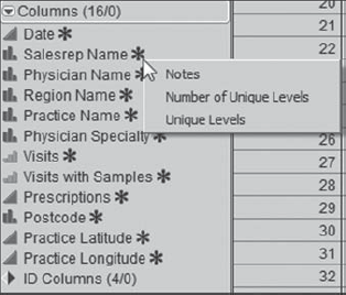
Also, you will note that in PharmaSales.jmp asterisks appear next to each variable name in the columns panel. For example, if you click on the asterisk next to Salesrep Name, a list showing the column properties associated with that variable appears, as shown in Exhibit 7.65. The script has placed two new properties in Column Info: Number of Unique Levels and Unique Levels.
Figure 7.65. List of Column Properties for Salesrep Name
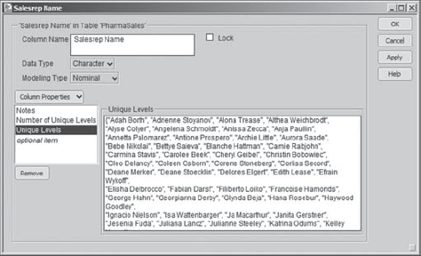
Click on Unique Levels. This opens the Column Info dialog, and the unique levels of Salesrep Name, namely the names of all the sales representatives, are shown in the text window (Exhibit 7.66).
Figure 7.66. Unique Levels for Salesrep Name, Shown in Column Info Dialog
The script Delete Unique Levels removes the column properties inserted by the Unique Levels script. If you find these scripts useful, you can copy them to other JMP tables.
7.8.2. Saving a Script to Create a Summary Data Table
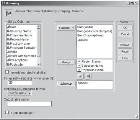
This section describes how you would save a script that creates a summary table to the parent data table. Recall that Rick created a summary data table from the data in PharmaSales.jmp (Exhibit 7.34) by selecting Tables > Summary and filling out the dialog as shown in Exhibit 7.67.
Figure 7.67. Dialog for Summary Table 1
When you run this summary dialog, in the resulting summary table you will see a script called Source. This is the script that creates the summary table. To run the summary from a script in the main data table, you need only copy the Source script to the parent data table, namely, to PharmaSales.jmp.
So, with PharmaSales.jmp active, run the dialog in Exhibit 7.67. In the summary table, click on the red triangle next to Source, choose Edit, and copy the script to the clipboard. Then, close the script window and make the data table PharmaSales.jmp active. In this data table, click on the red triangle next to PharmaSales in the data table panel (Exhibit 7.68) and choose New Property/Script.
Figure 7.68. New Property/Script Option in Data Table Panel

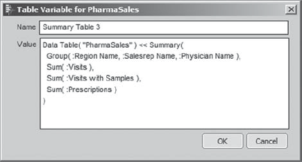
This opens a text window where you can paste the Source script. Here, we have named the script Summary Table 3 to distinguish it from the two summary scripts that are already saved. The text window is shown in Exhibit 7.69. Just to be sure that this works, click OK and run the script.
Figure 7.69. Summary Table Script Window
7.8.3. Constructing a Year-to-Date Summary Table
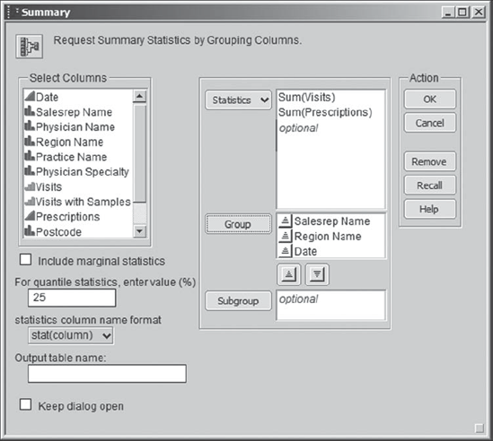
In this section, we give the details of how Rick accumulates his outcome variables on a year-to-date basis as required in the data table given by the script Summary Table 2. To begin, Rick makes his main table, PharmaSales.jmp, the active table. He first needs to aggregate Prescriptions and Visits for each sales representative each month. In other words, he wants to sum these two variables over the physicians serviced by each sales representative. To do this, Rick selects Tables > Summary, completes the launch dialog as shown in Exhibit 7.70, and then clicks OK.
Figure 7.70. Summary Table Launch Dialog
In the resulting data table, Rick sees a column called N Rows. This is the total number of rows in PharmaSales.jmp for each sales representative in the given month. Rick realizes that this is just the number of physicians assigned to the given sales representative. For this reason, he renames the N Rows column to Number of Physicians (Exhibit 7.71).
Figure 7.71. Partial View of Summary Data Table

At this point, Rick wants to add year-to-date sums of Visits and Prescriptions to this data table. He will do this by creating two new columns, called Visits YTD and Prescriptions YTD, using formulas. His plan is to base year-to-date sums on the Date column, summing only one row for May, two rows (May and June) for June, and so on. We will not describe how these formulas are defined in detail, but we sketch Rick's approach in the context of the formula for Visits YTD.
First, by double-clicking in the empty column header area to the right of Sum(Prescriptions), Rick opens a new column. He names this new column Visits YTD. Then he right-clicks in the header area to open the context-sensitive menu, where he chooses Formula. This opens the formula editor window. Under Table Columns, Rick selects Date. This enters Date into the formula editor.
Just a reminder about dates in JMP: Any date is stored as a continuous value representing the number of seconds since January 1, 1904. Available under Column Info, the date formats translate the number of seconds into recognizable date formats such as the m/y (month/year) format used for Date in PharmaSales.jmp.
Back to Rick, who has Date entered into the formula editor. Rick wants to define a partial sum for each value of Date. To do this, he will use the Match function, available under the Conditional grouping. But he would prefer not to have to type each of the dates into the Match function in order to define the partial sum that is appropriate for that value of Date. So, he uses a JMP shortcut. With Date in the formula editor and selected (there should be a red rectangle around it), Rick holds down the shift key as he clicks on Conditional in the list of Functions (grouped). At that point, he releases the shift key and selects Match (Exhibit 7.72).
Figure 7.72. Formula Editor Showing Match Function
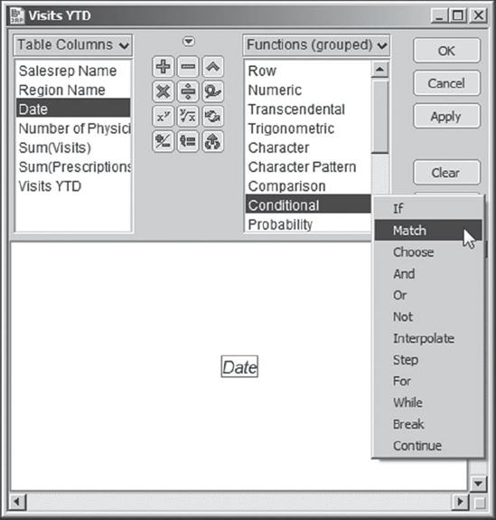
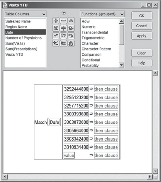
Holding down the shift key while choosing Conditional causes JMP to list each possible value of Date as a conditional argument to the Match function. The resulting function template appears as shown in Exhibit 7.73. Each date is shown using its internal representation as the number of seconds since January 1, 1904. However, since the dates are listed in increasing order, it is clear to Rick that the value 3292444800 represents May 2008, 3295123200 represents June 2008, and so on.
Figure 7.73. Match Function with All Values of Date as Conditional Arguments
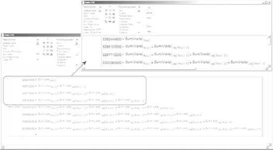
Now Rick can enter the partial sum functions for each date. The finished formula is shown in Exhibit 7.74, where we have enlarged the first four sums for visibility. For May 2008, the partial sum is simply the value of Sum(Visits) for the current row. Rick enters this into the then clause rectangle by selecting the then clause text area, selecting Sum(Visits) under Table Columns, and, while it is selected (surrounded by the red rectangle) in the formula editor, clicking on Row under Functions (grouped) and choosing Subscript, then going to Row again and choosing Row (to fill the Subscript box). The formula tells JMP that if the month is May 2008, then Visits YTD should return the value of Sum(Visits) in the current row.
To construct the formula for June, Rick begins by copying his formula for May, which is Sum(Visits) subscripted by Row( ), into the formula rectangle for June 2008. Then he clicks a plus sign and defines the second summand shown in Exhibit 7.74. Here, for the subscript, he selects repeatedly under the Row formula grouping: first, Subscript, next Lag, then Row. He continues building his partial sums in this fashion, entering appropriate values for the lag argument. He uses a similar approach to construct Prescriptions YTD.
Figure 7.74. Formula for Visits YTD
To view these formulas on your screen, run the script Summary Table 2 in PharmaSales.jmp. In the columns panel, click on the plus sign next to Visits YTD or Prescriptions YTD.