8.6. Modeling Relationships

The data exploration up to now has revealed several relationships between Xs, which may be Hot Xs, and the two Ys of interest, MFI and CI. At this point, Carl and the team embark on the task of modeling the relationships in a multivariate framework.

Carl formulates a plan and explains it to his teammates. First, they will develop two models, one that relates the Xs to MFI and one that relates the Xs to CI. By examining the results, they will determine Hot Xs for each response and reformulate the models in terms of these Hot Xs. Then, they will use the profiler to simultaneously optimize both models, finding the best settings for the entire collection of Hot Xs. Once this is accomplished, they will find optimal operating ranges for these Xs. They will then investigate how variation in the Hot Xs propagates to variation in the Ys.

8.6.1. Dealing with the Preliminaries

Carl struggles with the issue of what to do with the four MFI outliers. He realizes that he could include these four rows in the model development process and, once a model is selected, check to see if they are influential (using visual techniques and statistical measures such as Cook's D). Or, he could just develop models without them.

Looking back at the histograms and control charts for MFI, Carl sees that they are very much beyond the range of most of the MFI measurements. More to the point, they are far beyond the specification limits for MFI. The fact that they are associated with extremely low yields also points out that they are not in a desirable operating range.

Since Carl is interested in developing a model that will optimize the process, he needs a sound model over that desirable operating range. The outliers will not help in developing such a model, and, in fact, they might negatively affect this effort. With this as his rationale, Carl decides to exclude them from the model development process.

To exclude and hide the four outliers, Carl runs Distribution with Yield as Y, Columns. In the box plot part of the plot, he drags a rectangle to contain the four points. In the plot, he right-clicks and selects Row Exclude (see Exhibit 8.49). He right-clicks once more and selects Row Hide. He checks in the rows panel of the data table to make sure that four points are Excluded and Hidden. (If your four outlier rows are still selected, you can simply select Row Exclude and Row Hide; there is no need to select the points once more. Alternatively, whether they are selected or not, you can run the script Exclude and Hide Outliers.)

In the interests of expediency for subsequent analyses, Carl decides to store the specification limits for MFI and CI in the data table. He right-clicks in the MFI column header and chooses Column Info. In the Column Info dialog, from the Column Properties list, he chooses Spec Limits (Exhibit 8.50).

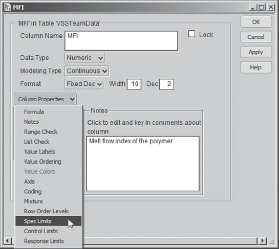
He fills in the text boxes as shown in Exhibit 8.51, recording that the target is 195, with lower and upper specification limits of 192 and 198, respectively. He clicks OK. Carl proceeds in a similar fashion for CI, recording only a lower specification limit of 80. (If you wish to simply insert these by means of a script, run the script Spec Limits.)

8.6.2. Plan for Modeling

Now Carl has another decision to make—how to build a model? There are a number of options: Fit Model, with manual elimination of inactive terms, Fit Model using the Stepwise personality for automated variable selection, or the Screening platform. Carl thinks: "Wow, something new—I have never tried screening!" The idea of using this platform intrigues him.

He decides to get some advice about the screening platform from his mentor, Tom. Over lunch together, Tom explains that the screening platform was developed to analyze the results of a two-level regular fractional factorial experiment and that it is in this situation where its performance is best. That being said, Tom tells Carl that the screening platform may also be useful when exploring observational data.

Tom also mentions that nominal variables should not be included when using the screening platform, since it will treat them as if they were measured on a continuous scale. He warns Carl to check the viability of the predictors he obtains through Screening by running Fit Model on the same selection. It is at this point that Carl might want to also include his nominal variables.

The conversation moves to a discussion of the nominal factors, Quarry and Shift. Keeping in mind that the purpose of this modeling effort is to find optimal settings for the process variables, Tom suggests that perhaps it does not make sense to include Shift in this modeling effort. None of the exploratory analysis to date has suggested that Shift affects the responses MFI and CI.

Just to ensure that multivariate relationships have not been overlooked, after lunch Carl pulls out his computer, and they conduct a quick partition analysis (Analyze > Modeling > Partition). They conclude that Shift and Quarry seem to have very little impact on MFI, where SA, M%, and Xf seem to be the drivers, and little impact on CI, where Xf and SA appear to be the drivers. (We encourage you to explore this on your own.)

Given that Shift cannot be controlled, and armed with the knowledge that it does not appear to affect either response in a serious way, Carl is content not including Shift in the modeling. But what about Quarry, which could be controlled if need be? Tom suggests that Carl add Quarry and its interactions with other linear terms once potential predictors have been identified using the screening platform.

Carl is comfortable with this plan. For each of MFI and CI, he will:

• Identify potentially active effects among the continuous Xs using Screening.

• Use these as effects in a Fit Model analysis.

• Add Quarry and its interactions with the linear terms identified by Screening to the effects list for the Fit Model analysis.

• Reduce the effect list to obtain a final model.

He will then use these final models to find settings of the Hot Xs that simultaneously optimize both MFI and CI. At that point, he also hopes to quantify the anticipated variability in both responses, based on the likely variation exhibited by the Hot Xs in practice.

8.6.3. Using Screening to Identify Potential Predictors

Carl and his teammates are ready for some exciting analysis. Carl selects Analyze > Modeling > Screening. He populates the launch dialog as shown in Exhibit 8.52.

Carl clicks OK. The report that appears is partially shown in Exhibit 8.53. Carl saves its script with the default name Screening. There are two analyses presented side-by-side, one for MFI and one for CI. Note that the disclosure icon for the CI report is closed in Exhibit 8.53. Carl intends to use these reports to develop separate models for these two responses. (If you are running this analysis on your own, please note that your p-values will not exactly match those shown in Exhibit 8.53. This is because the p-values are obtained using a simulation. However, the values should be very close, usually only differing in the third decimal place.)

At this point, Carl reviews his notes on the screening platform and has another quick discussion with Tom. The screening platform fits as many terms as possible to a response to produce a saturated model. Because there are 106 rows (recall that four outliers were excluded), 105 separate terms or effects can be estimated.

Screening includes terms by first introducing linear terms, or main effects (the six factors), then all two-way interactions and squared terms in these six factors (there are 21 such terms), then three-way interactions and cubic terms, and so on, until no more effects can be fit. Second-order terms are introduced in an order determined by the significance of first-order terms, and this thinking continues with higher-order terms. In Carl's example, a large number of three-way interactions and cubic terms are included. This can be seen by examining the entries in the Term column.

The Screening for MFI report lists the 105 possible model terms. Carl recalls from his training that the analysis philosophy behind the Screening platform is that of effect sparsity, which is the idea that only a few of the potential or postulated model terms will actually be important in explaining variation in the response.^[] These important terms are often called active effects. The simulated p-values provide a means of classifying terms into signal or noise, and effect sparsity would lead us to always expect relatively few active terms.

The measure of the effect of a term is represented by its contrast. If the data were from a two-level orthogonal design, the contrast would be the effect of the factor—the difference between the mean at its high setting and the mean at its low setting. (See the JMP Help documentation for further details.)

The test statistic is Lenth's t-Ratio. Two types of p-values are provided. Now, as Carl was reminded in his recent talk with Tom, it is important to keep in mind that these p-values are obtained using simulation and that different, though very similar, p-values will be obtained when the analysis is rerun. For example, when you run the Screening script that Carl saved, you will see p-values that differ slightly from those shown in Exhibit 8.53.

But how do the two types of p-values, individual p-values and simultaneous p-values, differ? The individual p-values are analogous to p-values obtained for terms in a multiple linear regression. (Note that in the screening platform JMP highlights each term that has an individual p-value less than 0.10.) Now, with 105 terms, each being tested at a 5 percent significance level, a sizable number could easily appear to be significant just by chance alone. This is why the simultaneous p-values are important. The simultaneous p-values are adjusted for the fact that many tests are being conducted.

Carl remembers that in his training Tom discussed these two types of p-values in terms of Type I (false positive) and Type II (false negative) errors. A false positive amounts to declaring an effect significant when it is not. A false negative results in declaring an effect not to be significant when, in fact, it is. Neither of these errors is desirable, and there is always a trade-off between them: A false positive can result in costs incurred by controlling factors that don't have an effect; a false negative can overlook factors that are actually part of the causal system and that could be manipulated to produce more favorable outcomes. Tom believes that any inactive factors that are incorrectly included in a model have a way of exposing themselves in later analysis, so his recommendation here is to minimize false negatives at the expense of false positives.

Now, to relate these errors to the p-values, Carl realizes that using the Individual p-values might result in false positives, while using the Simultaneous p-values might result in false negatives. He resolves to strike a balance between these two possibilities.

With this in mind, Carl looks at the Screening for MFI report and wishes that the p-values could be sorted. Then he remembers that by right-clicking in a section of a report, JMP often provides options that users would like to have. When he right-clicks in the Screening for MFI report, to his delight, a menu appears with the option Sort by Column (Exhibit 8.54). Carl immediately clicks on that option, which opens a Select Columns menu (also shown in Exhibit 8.54), where he chooses to sort on the report column Individual p-Value.

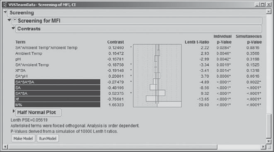
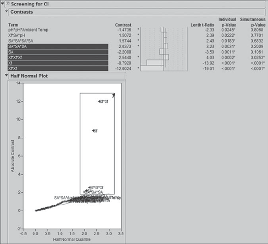
The default sort is in descending order, which turns out to be very convenient. This is because the sorting pushes the significant effects to the bottom of the list, where there is a Half Normal Plot and a button to Make Model. Exhibit 8.55 shows the bottom part of the list of 105 terms for MFI, along with the Make Model (and Run Model) buttons.

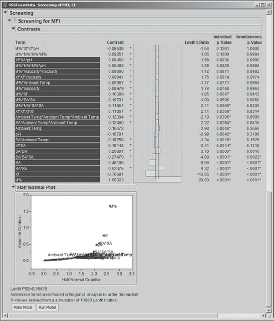
Carl studies the information in this report. He checks the sizes of the contrasts, using the bar graph shown to the right of the contrasts. Although his data are observational, the size of the contrast does give an indication of the practical importance of the corresponding effect. Carl also studies the Half Normal Plot, which shows the absolute values of the contrasts plotted against quantiles for the absolute value of the normal distribution. Terms that contribute random noise will fall close to their corresponding quantiles, and hence close to the line in the plot. Significant terms will fall away from the line and toward the upper right of the plot.

Carl resizes the Half Normal Plot to lengthen the vertical axis. To do this, he places his cursor over the horizontal axis and positions it so that a double arrow appears. Then, he clicks and holds, dragging the plot downward (just like making an application window bigger in Windows or OS-X). The resized plot is shown in Exhibit 8.56.

Looking at this plot, Carl decides that he will select all effects with Absolute Contrast values equal to or exceeding that of SA*SA*SA. He selects these in the plot by dragging a rectangle around them, as shown in Exhibit 8.57. He could also have selected them by control-clicking effect names in the report.

The five selected effects are shown in Exhibit 8.58. Carl notes that these include all of the effects with Simultaneous p-Values less than 0.05. Carl could have considered more effects, but his sense from the p-values and the Half Normal Plot is that his selection will include the terms that are likely to have an effect on the process. With this choice, Carl thinks that he has achieved a reasonable balance between overlooking potentially active terms and including terms that do not contribute. (We encourage you to investigate models that contain more effects; these are quite interesting.)

8.6.4. Obtaining a Final Model for MFI

Carl clicks the Make Model button located below the Half Normal Plot. This opens the Selected Model dialog, shown in Exhibit 8.59. The effects that were selected in the screening platform are entered in the Construct Model Effects text box. Carl saves this dialog as Screening Model for MFI.

Carl is about to run this model when he remembers Quarry. The plan was to enter Quarry as an effect in the Construct Model Effects list and also to add all two-way interactions with Quarry. So, Carl clicks on Quarry in the Select Columns list and clicks Add to place it in the Construct Model Effects list. Then, to add all two-way interactions with Quarry, he selects Quarry in the Select Columns list, selects M%, Xf, and SA in the Construct Model Effects list, and clicks Cross. Carl also changes the Emphasis in the drop-down at the top right of the dialog to Effect Screening to fine tune the output in the report. The resulting Selected Model dialog is shown in Exhibit 8.60. Carl saves this dialog as Model for MFI with Quarry.

Now Carl clicks on Run Model. In the report, shown in Exhibit 8.61, the Actual by Predicted plot indicates that the model fits the data well. Carl realizes that he could also check the residuals using the traditional Residual by Predicted Plot, which can be obtained by selecting Row Diagnostics > Plot Residual by Predicted from the red triangle. But this latter plot is essentially a rotated version of the Actual by Predicted Plot, so Carl forgoes the pleasure.

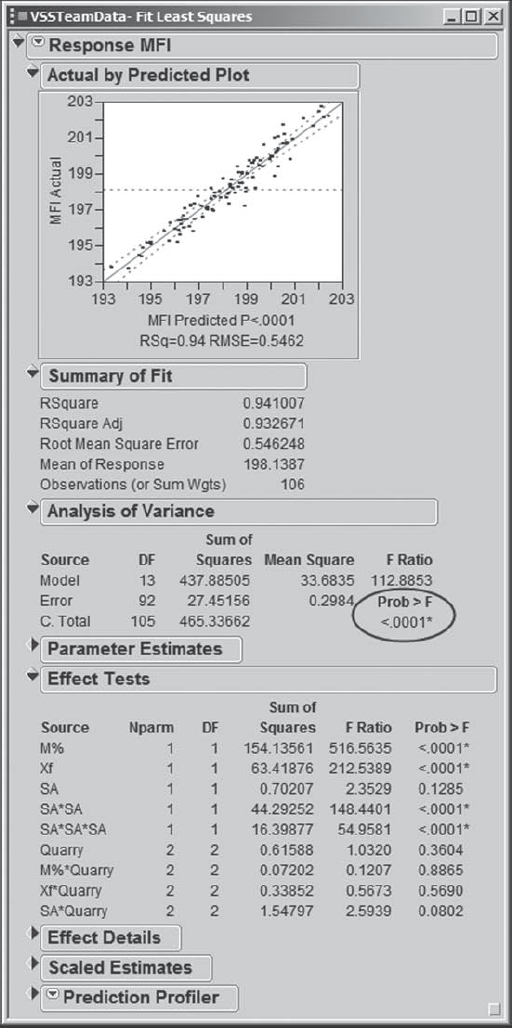
The model is significant, as indicated by the Prob > F value in the Analysis of Variance panel. The Effect Tests panel indicates that there are a number of effects in the model that are not statistically significant. Carl decides to reduce the model before doing further analysis.

Carl could remove effects one by one, refitting the model each time, since the Prob > F values will change every time the model is refit. But, in the training that he had with Tom, Tom suggested the following approach, which he prefers especially for models with many terms. Place the Selected Model dialog and the Fit Least Squares report side-by-side. Then remove all effects with Prob > F greater than 0.20.

This seemed a bit odd to Carl at the time, but Tom explained that as you remove terms one-by-one from a model, the Prob > F values as a whole tend to drop. So you may be painting an unrealistic picture of which terms are truly significant. Tom pointed out that removing terms in a block partially overcomes this issue and might actually be more appropriate when dealing with multiple tests.

Carl decides to follow Tom's advice. He places the Selected Model dialog and the Fit Least Squares report side-by-side, as shown in Exhibit 8.62. He identifies the effects that have Prob > F values greater than 0.20 and are not involved in higher-order terms or interactions. Only two terms qualify: M%*Quarry and Xf*Quarry. Carl removes these terms from the Selected Model dialog by selecting them in the Construct Model Effects list, then clicking the Remove button above the list.

He reruns the model (Exhibit 8.63). The interaction term SA*Quarry has a Prob > F value of 0.1011, and the main effect Quarry has a Prob > F value of 0.2718. Carl had been thinking about a 0.10 cut-off for Prob > F values, so as to minimize the risk of overlooking active effects. He is undecided as to whether to leave the borderline interaction, and hence the main effect, in the model or to remove both effects. Finally, he comes down on the side of not overlooking a potentially active factor. He can always remove it later on.

He saves the dialog window that created this model, shown in Exhibit 8.64, as Reduced Model for MFI. He notes that the Hot Xs for MFI are M%, Xf, and SA, with Quarry potentially interesting as well.

Happy with this model, Carl returns to the report shown in Exhibit 8.63. He wants to save the prediction formula given by this model for MFI to the data table. He knows that he will want to simultaneously optimize both MFI and CI, so it will be necessary to have both prediction equations saved in his table. To add a column containing the prediction formula to the data table, Carl clicks the red triangle at the top next to Response MFI and selects Save Columns > Prediction Formula. (Alternatively, you can run the script Prediction Formula for MFI.)

A new column called Pred Formula MFI appears in the data table. In the columns panel next to the column's name, there is a plus sign, indicating that the Pred Formula MFI column is given by a formula. Carl clicks on the plus sign to reveal the formula, which is shown in Exhibit 8.65. After a quick look, he closes the formula box by clicking Cancel. He also notes the asterisk next to the plus sign. He clicks on it to learn that the Spec Limits property that he previously defined for MFI has been included as a Column Property for the prediction formula. How nifty!

Before continuing, we note the following points:

8.6.5. Obtaining a Final Model for CI

Now Carl conducts a similar analysis for CI. He returns to the Screening report, sorts the Terms in the Screening for CI panel by Individual p-Value, and examines the Half Normal Plot. As he did for MFI, in the plot he selects the effects that appear to be significant using a rectangle, shown in Exhibit 8.66. This selects the bottom five effects in the Terms list: SA, Xf, a quadratic term in Xf, a cubic term in Xf, and a cubic term in SA.

Carl notes that his selected effects include all of the effects with Simultaneous p-Values below 0.20. He checks the effects in the Term list immediately above the ones that he has chosen. Although some of these are two-way interactions, a number are third- and fourth-degree terms. Since fourth-degree terms are rarely important, and since they do not appear significant in the Half Normal Plot, he is content to proceed with the five effects that he has chosen.

He clicks Make Model. In the interest of maintaining model hierarchy, he adds the SA*SA term. He does this by selecting SA in the Select Columns list as well as in the Construct Model Effects list and clicking Cross. He saves this dialog as Screening Model for CI. Next, Carl adds Quarry and the two-way interactions of Quarry with Xf and SA to the model. He saves this script as Model for CI with Quarry.

Reducing this model by eliminating terms where Prob > F exceeds 0.20 results in the elimination of only SA*Quarry. When Carl reruns the model, it seems clear that SA*SA and SA*SA*SA should be removed, based on their large Prob > F values. When he reruns this further-reduced model, he notes that the Xf*Quarry interaction has a Prob > F value of 0.1423 and that the Quarry main effect has a Prob > F value of 0.954. He considers this to be sufficient evidence that neither the interaction nor the main effect is active. So, he removes these two terms as well. Although SA is now significant only at 0.1268, he decides to retain it in the model.

He checks the resulting model and notes that it appears to fit well. He concludes that the Hot Xs for CI are Xf and SA. Finally, he saves the resulting model dialog as Reduced Model for CI (see Exhibit 8.67) and saves the prediction formula to the data table. (The script Prediction Formula for CI will also save this formula to the data table.)