
9.5. Modeling Relationships: Logistic Model
Recall that Mi-Ling intends to explore three modeling approaches: logistic regression, recursive partitioning, and neural nets. She considers using discriminant analysis, but recalls that discriminant analysis requires assumptions about the predictor variables—for each group, the predictors must have a multivariate normal distribution, and unless one uses quadratic discriminant analysis, the groups must have a common covariance structure. Thinking ahead to her test campaign data, Mi-Ling notes that some of her predictors will be nominal. Consequently, discriminant analysis will not be appropriate, whereas logistic regression will be a legitimate approach.
Mi-Ling begins her modeling efforts with a traditional logistic model. But before launching into a serious logistic modeling effort, Mi-Ling decides that she wants to see how a logistic model, based on only two predictors, might look. She begins by fitting a model to only two predictors that she chooses rather haphazardly.
Once she has visualized a logistic fit, she proceeds to fit a logistic model that considers all 30 of her variables as candidate predictors. She uses a stepwise regression procedure to reduce this model.
9.5.1. Visualization of a Two-Predictor Model
Since she will use only the training data in constructing her models, Mi-Ling copies the values in the row state variable Training Set to the row states in the data table CellClassification_2.jmp. As she did earlier, she clicks on the star to the left of Training Set in the columns panel and selects Copy to Row States. In the rows panel, she checks that 222 rows are Excluded and Hidden.
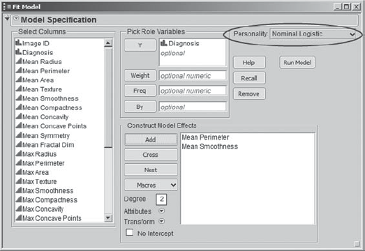
To be able to visualize a logistic model in a simple situation, Mi-Ling begins by fitting a model to only two predictors, Mean Perimeter and Mean Smoothness, which she chooses simply because these variables have caught her attention. She selects Analyze > Fit Model and enters Diagnosis as Y. When she does this, she notices that JMP instantly inserts Nominal Logistic as the Personality for this model. In Fit Model, JMP provides a number of personalities—these are essentially different flavors of regression modeling. In this case, JMP notices that Diagnosis is nominal and that, consequently, a logistic regression model is appropriate. In the Select Columns list on the left, she selects Mean Perimeter and Mean Smoothness and clicks on the Add button to the left of the Construct Model Effects box (Exhibit 9.63). She saves the script for the launch dialog to the data table as Logistic – Two Predictors.
Figure 9.63. Launch Dialog for Logistic Fit with Two Predictors
When she clicks OK, she sees the Nominal Logistic Fit report shown in Exhibit 9.64. She is pleased to see that the Whole Model Test is significant and that the p-values in the Effect Likelihood Ratio Tests portion of the report, given under Prob > ChiSq, indicate that both predictors are significant.
Figure 9.64. Fit Nominal Logistic Report for Two-Predictor Model

Now Mi-Ling is anxious to see a picture of the model. She remembers that for one predictor a logistic model looks like an S-shaped curve that is bounded between 0 and 1. She wonders what the surface for a model based on two predictors will look like. She clicks on the red triangle at the top of the report and chooses Save Probability Formula (Exhibit 9.65).
Figure 9.65. Options for Fit Nominal Logistic

This saves four formula columns to the data table. The two columns that most interest Mi-Ling are Prob[M] and Most Likely Diagnosis. The column Prob[M] gives the predicted probability that a mass is malignant (of course, Prob[B] = 1 − Prob[M]). Mi-Ling notes that all of these predicted values are between 0 and 1, as they should be. She clicks on the plus sign that follows Prob[M] in the columns panel to see the formula (Exhibit 9.66). The formula is a logistic function applied to Lin[B], which in turn is a linear function of the two predictors. So Prob[M] is itself a nonlinear function of the two predictors.
Figure 9.66. Formula for Prob[M]

Mi-Ling also checks the formula for Most Likely Diagnosis (Exhibit 9.67). She figures out that the formula says, "If the larger of Prob[B] and Prob[M] is Prob[B], then predict B. If the larger of Prob[B] and Prob[M] is Prob[M], then predict M." So the formula is predicting the outcome class that has the largest predicted probability. That means that B is assigned if and only if Prob[B] exceeds 0.50, and similarly for M.
Figure 9.67. Formula for Most Likely Diagnosis

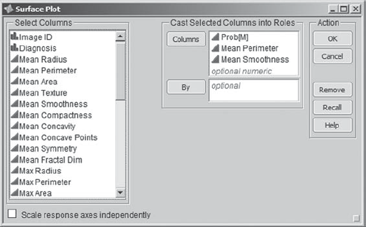
To construct a picture of the prediction surface, Mi-Ling selects Graph > Surface Plot. Since she wants to see how Prob[M] varies based on the values of Mean Perimeter and Mean Smoothness, she populates the launch dialog as shown in Exhibit 9.68.
Figure 9.68. Launch Dialog for Surface Plot
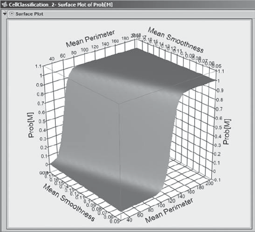
When she clicks OK, she sees the surface plot shown in Exhibit 9.69. She takes her cursor over to the plot, which she then rotates by holding down the left mouse button. This allows her to see the surface from various angles. She sees that the surface has an S shape, with all Prob[M] values between 0 and 1, as they should be.
Figure 9.69. Surface Plot of Prob[M]
But what about the individual points? She would like to display their predicted values, along with their Diagnosis markers and colors, on the plot. To plot the points, she goes to the Dependent Variables panel beneath the plot. She sees that Prob[M] is the only formula entered, as it should be. To the right of Prob[M], in the second column, called Point Response Column, she chooses Prob[M] (see Exhibit 9.70, where the markers have been made solid and enlarged for visibility). This has the effect of plotting Prob[M] values for the points on the three-dimensional grid. Since the surface that is plotted is the prediction surface, all the predicted values fall on that surface.
Figure 9.70. Surface Plot of Prob[M] with Points and Grid

However, since the points are colored and marked according to the actual outcome, Mi-Ling easily sees the points corresponding to malignant masses—they are depicted by red triangles. She wonders, "Are most of these predicted to be malignant?" Well, a mass is predicted to be malignant if Prob[M] exceeds 0.50. On the far right in the Dependent Variables panel, Mi-Ling notices a text box labeled Grid Value and, below it, a Grid slider. The Grid Value is already set to 0.5. Mi-Ling checks the box to the right of the Grid slider, which inserts a grid in the plot at Prob[M] = 0.5 (Exhibit 9.70).
She sees that most points that correspond to malignant masses (identified by triangles) are above the grid at 0.5. However, a number fall below; these correspond to the malignant masses that would be classified as benign, which is a type of misclassification error. Similarly, most benign points (plotted as circles) are below the grid, but again, a few are above it; these correspond to benign masses that would be classified as malignant, another type of misclassification error. Mi-Ling saves the script for the plot as Surface Plot – Two Predictors.
Mi-Ling concludes that the model is not bad, but the two types of misclassification errors appear consequential. She realizes that an easy way to quantify the misclassification errors is to compare Most Likely Diagnosis with the actual values found in Diagnosis using Fit Y by X. She selects Analyze > Fit Y by X, where she inserts Most Likely Diagnosis as Y, Response and Diagnosis as X, Factor. She clicks OK and obtains the report shown in Exhibit 9.71.
Figure 9.71. Contingency Report for Two Predictor Model

In the mosaic plot, the two circled areas indicate misclassifications. The circled (blue) area above B indicates masses that were benign but that were classified as malignant, while the circled (red) area above M indicates masses that were malignant but that were classified as benign.
Mi-Ling finds the contingency table informative. From the Total % value, she sees that malignant masses are classified as benign 6.92 percent of the time and benign masses are classified as malignant 3.17 percent of the time.
To better focus on Count and Total %, Mi-Ling sees that she can remove Row % and Column % from the contingency table by deselecting these options from the red triangle menu provided next to Contingency Table. But she realizes that in her analyses she will be constructing several contingency tables, and would prefer not to have to deselect these options every time. In short, she would like to set a preference relative to what she sees when she runs a contingency analysis.
She closes the Contingency report. Then, she selects File > Preferences, selects Platforms, and then selects the Contingency platform. In the list of options, she deselects Row % and Col %. She clicks OK. Then she reruns her Fit Y by X analysis by selecting Analyze > Fit Y by X and clicking the Recall button in the Action column, followed by OK. She obtains the output in Exhibit 9.72. Mi-Ling saves the script for this analysis as Contingency – Two Predictors.
Figure 9.72. Contingency Report Showing Modified Table

In the revised Contingency Table, Mi-Ling easily sees that masses that are actually malignant are classified as benign in 24 instances, while masses that are benign are classified as malignant in 11 instances. In other words, there are 24 false negatives and 11 false positives. The overall misclassification error is 35 (24 + 11) divided by 347, or 10.1 percent. This is not very good, but Mi-Ling realizes that she did not choose her two predictors in any methodical way. Yet, this exercise with two predictors has been very useful in giving Mi-Ling insight on logistic modeling.
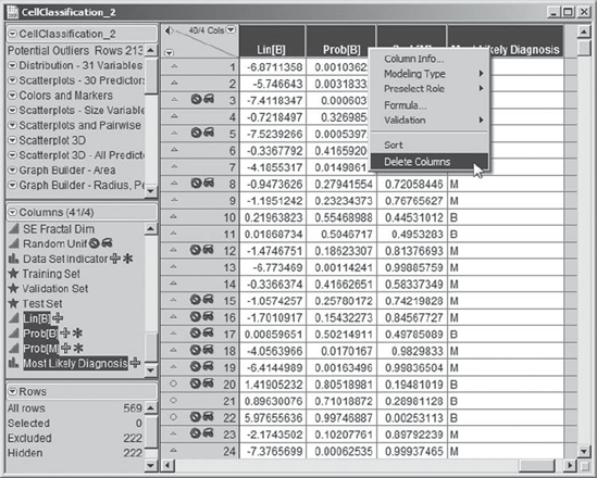
At this point, Mi-Ling is ready to get serious about model construction. She sees no further need for the four columns that she has saved to the data table, given that she can reproduce them easily enough by running the script Logistic – Two Predictors, running the model, and saving the probability formula columns. So, she deletes them. To do this, she selects all four columns, either in the data grid, as shown in Exhibit 9.73, or in the columns panel. She right-clicks in the highlighted area and selects Delete Columns. (If you are working along with Mi-Ling, please delete these columns in order to avoid complications later on.)
Figure 9.73. Deleting the Four Save Probability Formula Columns
9.5.2. Fitting a Comprehensive Logistic Model
9.5.2.1. GROUPING PREDICTORS
In fitting her models, Mi-Ling realizes that she will often want to treat all 30 of her predictors as a group. James showed her that JMP can group variables. When a large number of columns will be treated as a unit, say, as potential predictors, this can make analyzing data more convenient. She decides to group her 30 predictors.
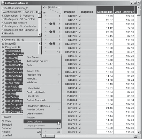
To do this, Mi-Ling selects all 30 of her predictors, from Mean Radius to SE Fractal Dim, in the columns panel. Then she right-clicks in the highlighted area and selects Group Columns, as shown in Exhibit 9.74.
Figure 9.74. Selection of Group Columns
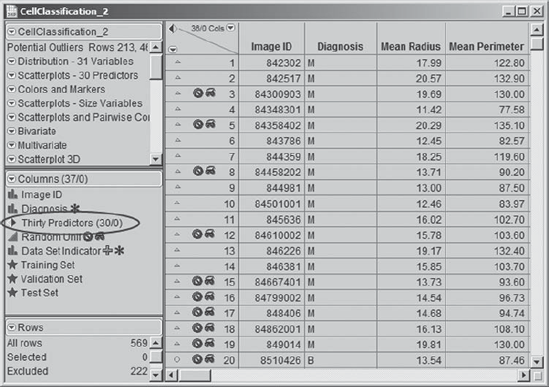
This has the effect of placing all 30 variables in a group designated by the name of the first variable. Mi-Ling double-clicks on the name that JMP has assigned—Mean Radius etc.—and changes it to Thirty Predictors (Exhibit 9.75). To view the columns in the group, Mi-Ling need only click the disclosure icon to the left of Thirty Predictors. (The script Group 30 Columns creates the group Thirty Predictors.)
Figure 9.75. Grouped Columns with Name Thirty Predictors
9.5.2.2. FITTING A STEPWISE LOGISTIC MODEL
Mi-Ling begins her thinking about fitting a logistic model by pondering the issue of variable selection. She has 30 potential predictors, and she knows that she could expand the set of terms if she wished. She could include two-way interactions (for example, the interaction of Mean Perimeter and Mean Smoothness), quadratic terms, and even higher-order terms. Even with only 30 predictors, there are well over one billion different possible logistic models.
To reduce the number of potential predictors that she might include in her logistic model, Mi-Ling decides to use stepwise regression. But which potential predictors should she include in her initial model? Certainly all 30 of the variables in her data set are potential predictors. However, what about interactions? She calculates the number of two-way interactions: (30 × 29)/2 = 435 (the same as the number of correlations). So including main effects and all two-way interactions would require estimating 30 + 435 + 1 = 466 parameters. Mi-Ling realizes that she has a total of 347 records in her training set, which is not nearly enough to estimate 466 parameters.
With that sobering thought, she decides to proceed with main effects only. She also plans to explore partition and neural net models; if there are important interactions or higher-order effects, they may be addressed using these modeling approaches.
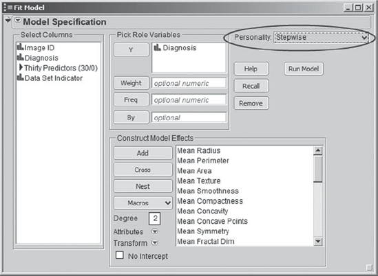
She checks to make sure that the row states for her training set have been applied. Once more Mi-Ling selects Analyze > Fit Model, where she enters Diagnosis as Y and all 30 of her predictors, which now have been grouped under the single name Thirty Predictors, in the Construct Model Effects box. Under Personality, she chooses Stepwise. This Fit Model dialog is shown in Exhibit 9.76. So that she does not need to reconstruct this launch dialog in the future, she saves its script as Stepwise Logistic Fit Model.
Figure 9.76. Fit Model Dialog for Stepwise Logistic Regression
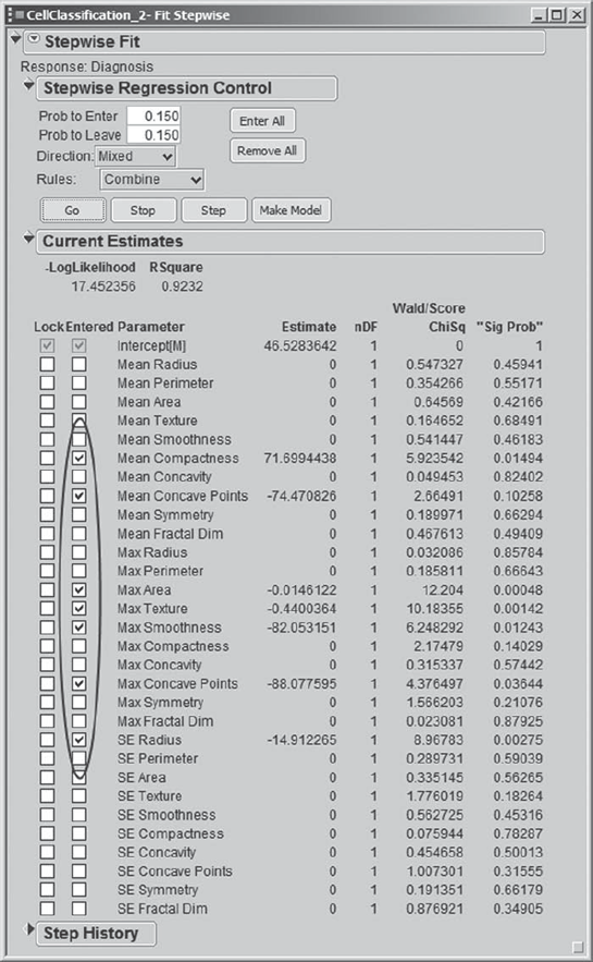
Clicking Run Model creates the Fit Stepwise report (Exhibit 9.77). In the Stepwise Regression Control panel, Mi-Ling can make stepwise selection choices similar to those available in linear regression analysis. Mi-Ling reminds herself that a forward selection procedure consists of sequentially entering the most desirable term into the model, while a backward selection procedure consists of sequentially removing the least desirable term from the model. The Current Estimates panel shows estimates of parameters and significance probabilities for the model under consideration at a given time.
Figure 9.77. Fit Stepwise Report

Because it tends to consider a large group of models, Mi-Ling decides to use a mixed procedure, meaning that each forward selection step will be followed by a backward selection step. To communicate this to JMP she sets Direction to Mixed in the Stepwise Regression Control panel. She also sets both the Prob to Enter and Prob to Leave values at 0.15. This has the effect that at a given step, only variables with significance levels below 0.15 are available to enter the model, while variables that have entered at a previous step but which now have significance levels exceeding 0.15 are available to be removed. The Stepwise Regression Control panel, as completed by Mi-Ling, is shown in Exhibit 9.78. She saves this in the script Stepwise Fit Report.
Figure 9.78. Stepwise Regression Control Panel for Logistic Variable Selection

When Mi-Ling clicks Go, she watches the Current Estimates panel as seven variables are selected (Exhibit 9.79). Alternatively, she could have clicked Step to see exactly how variables enter and leave, one step at a time.
Figure 9.79. Current Estimates Panel in Fit Stepwise
The Step History panel (Exhibit 9.80) gives a log of the sequence in which variables were entered and removed. Also provided are various statistics of interest. Mi-Ling thinks back to the fact that her training set contained two rows with unusually large values of SE Concavity. She sees that SE Concavity did not appear in the Step History and that it does not appear in the final model. In a way, this is comforting. On the other hand, it is possible that these rows were influential and caused SE Concavity or other predictors not to appear significant. At a future time, Mi-Ling may consider fitting a logistic model with these two rows excluded. For now, she continues with her current model.
Figure 9.80. Step History Panel in Fit Stepwise

To fit the seven-predictor model obtained using her training set, Mi-Ling clicks on Make Model in the Stepwise Regression Control panel. This creates a Stepped Model launch dialog containing the specification for Mi-Ling's seven-predictor model (the saved script is Stepwise Logistic Model).
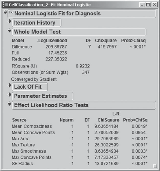
Finally, Mi-Ling clicks Run Model. The report (Exhibit 9.81) shows details about the model fit. The overall model fit is significant. The Effect Likelihood Ratio Tests show that all except one predictor is significant at the 0.01 level.
Figure 9.81. Fit Nominal Logistic Report for Stepwise Model
Mi-Ling clicks the red triangle in the report and chooses Save Probability Formula. Recall that this saves a number of formulas to the data table, including Prob[B] and Prob[M], namely, the probability that the tumor is benign or malignant, respectively, as well as a column called Most Likely Diagnosis, which gives the diagnosis class with the highest probability, conditional on the values of the predictors.
To see how well the classification performs on the training data, Mi-Ling selects Analyze > Fit Y by X. As before, she enters Most Likely Diagnosis as Y, Response and Diagnosis as X, Factor. The resulting mosaic plot and contingency table are shown in Exhibit 9.82. Of the 347 rows, only five are misclassified. She saves the script as Contingency – Logistic Model.
Figure 9.82. Contingency Report for Logistic Model Classification

Mi-Ling thinks this is great. But reality quickly sets in when she reminds herself that there is an inherent bias in evaluating a classification rule on the data used in fitting the model. Once she has fit her other models, she will compare them all using the validation data set. At this point, she closes the reports that deal with the logistic fit. She is anxious to construct and explore a model using recursive partitioning.