
8.4. Measurement System Analysis
As a general principle, measurement systems for key variables should always be evaluated before engaging in data collection efforts. Since measurement uncertainty or error is suspected as being part of the reason previous attempts to find root causes of the polymer problems failed, it is all the more important that Carl's team thoroughly study the measurement systems for all the variables identified by the process map.
Carl's team learns that recent routine MSAs indicate that CI; polymer weight, which forms the basis for the Yield calculation; SA; M%; pH; Viscosity; and Ambient Temp are being measured with very capable instruments and methods. However, the measurement systems for MFI and Xf have not been evaluated in the recent past. Furthermore, given how these measurements are made, the team realizes that they may be prone to problems.
8.4.1. MSA for MFI
MFI is measured using a melt flow meter during an off-line laboratory test. Four instruments are available within the laboratory to perform the test, and there are three different laboratory technicians who do the testing. There is no formal calibration for the instruments. When Carl's team members interview the technicians who perform the test, they get the impression that the technicians do not necessarily use a standardized procedure.
Carl meets with the technicians and their manager to discuss the desired consistency of the measurement process and to enlist their support for an MSA. He reminds them that for characteristics with two-sided specification limits, a guideline that is often used is that the measurement system range, measured as six standard deviations, should take up at most 10 percent of the tolerance range, which is the difference between the upper and the lower specification limits. Since the upper and lower specification limits for MFI are 198 and 192, respectively, the guideline would thus require the measurement system range not to exceed 10% × (198 − 192) = 0.6 MFI units.
Carl also mentions that there are guidelines as to how precise the measurement system should be relative to part-to-part, or process, variation: The range of variability of a highly capable measurement system should not exceed 10 percent of the part-to-part (or, in this case, the batch-to-batch) variability.
Given these guidelines, Carl suggests that an MSA for MFI might be useful, and the technicians and their manager agree. He learns from the technicians that the test is destructive. MFI is reported in units of grams per ten minutes. The protocol calls for the test to run over a half-hour period, with three measurements taken on each sample at prescribed times, although due to other constraints in the laboratory the technicians may not always be available precisely at these set times. Each of these three measurements is normalized to a ten-minute interval, and the three normalized values are averaged. From preparation to finish, a test usually takes about 45 minutes to run.
Using this information, Carl designs the structure for the MSA. Since the test is destructive, true repeatability of a measurement is not possible. However, Carl reasons, and the technicians agree, that a well-mixed sample from a batch can be divided into smaller samples that can be considered identical. The three technicians who perform the test all want to be included in the study, and they also want to have all four instruments included. Carl suggests that the MSA should be conducted using samples from three randomly chosen batches of polymer and that each technician make two repeated measurements for each batch by instrument combination.
This leads to 72 tests: 3 batches × 3 technicians × 4 instruments × 2 measurements. Since each test is destructive, a sample from a given batch of polymer will have to be divided into 24 aliquots for testing. For planning purposes, it is assumed that the MSA design will permit three tests to be run per hour, on average, using three of the four instruments. This leads to a rough estimate of 24 hours for the total MSA. With other work intervening, the technicians conclude that they can finish the MSA comfortably in four or five workdays.
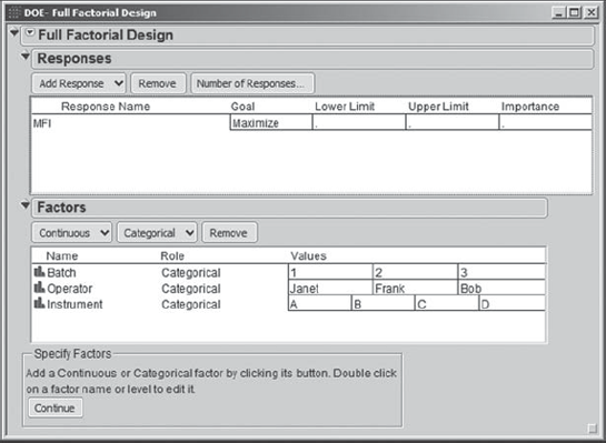
Next, Carl designs the experiment for the MSA. To do this, he selects DOE > Full Factorial Design. The resulting dialog window is shown in Exhibit 8.18.
Figure 8.18. DOE Full Factorial Design Dialog

Carl double-clicks on the response, Y, and renames it MFI. He notes the default goal of Maximize that JMP specifies. Since this is an MSA, there is no optimization goal relative to the response. He decides to simply leave this as is, since it will not affect the design. Next, by clicking on the Categorical button under Factors, he adds two three-level categorical factors and one four-level categorical factor. He renames these factors and specifies their values as shown in Exhibit 8.19.
Figure 8.19. DOE Full Factorial Design Dialog with Response and Factors Specified
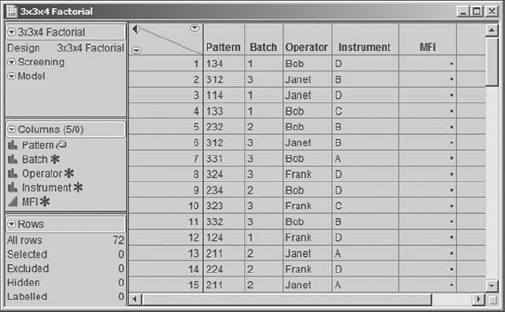
Carl then clicks Continue. He notes that the design, as specified so far, consists of 36 runs. Carl sees from the default specification that the Run Order will be randomized. Since two samples should be run at each of these 36 settings, he inserts a value of 1 in the box for Number of Replicates, as shown in Exhibit 8.20. Then he clicks Make Table and the design table, partially shown in Exhibit 8.21, appears. (Note that your table will likely appear different due to the fact that the run order is randomized.)
Figure 8.20. DOE Full Factorial Design Output Options
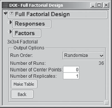
Figure 8.21. MSA Design Table
Carl notices that the DOE – Full Factorial Design dialog remains open; this is useful in case changes need to be made to the design that has been generated. As mentioned earlier, the runs are randomized. To the extent possible, the experiment will be run in this order. When JMP creates this design, it assumes that the goal is to model or optimize a process, so it automatically saves two scripts, Screening and Model, to the data table. But, since the data are being gathered for a measurement system analysis, Carl realizes that these scripts are not appropriate, and so he deletes them.
The technicians conduct the experiment over the course of the next week and enter their results into the data table that Carl has prepared. This table, containing the design and results, is called MSA_MFI_Initial.jmp and is partially shown in Exhibit 8.22.
Figure 8.22. Partial View of Data Table for Initial MFI MSA

Carl's team regroups to analyze the data. With this data table as the active window, Carl uses the JMP MSA platform, selecting Graph > Variability/Gauge Chart. He populates the dialog as shown in Exhibit 8.23 and clicks OK. Carl reflects for a moment on how easy it was to include Instrument as part of the analysis—traditional gauge R&R studies are usually limited to estimating variability due to operators and parts. The Variability/Gauge Chart platform makes including additional sources of variability trivial.
Figure 8.23. Launch Dialog for MFI MSA

In the menu obtained by clicking on the red triangle, he selects, one by one, Connect Cell Means, Show Group Means, and Show Grand Mean. This allows Carl and his teammates to get a sense of the variability between Batches, between Instruments, and between Operators. He deselects the St Dev Chart option, realizing that sufficient information on spread is given by the vertical distance between the two points in each cell. The resulting Variability Chart is shown in Exhibit 8.24. He saves the script with the name Variability Chart.
Figure 8.24. Variability Chart for Initial MFI MSA

It is immediately apparent from the variability chart that some sample measurements can vary by as much as three units when being measured by the same Operator with the same Instrument. For example, see Bob's measurement of Batch 3 with Instrument D. Carl clicks on these two points while holding down the shift key to select both. (Alternatively, he could draw a rectangle around them.) Then he goes to the data table, where he sees that the two rows have been selected. To create a table consisting of only these two rows, Carl right-clicks on Selected in the rows panel, as shown in Exhibit 8.25, and chooses Data View. This creates a data table containing only Bob's two measurements for Batch 3 with Instrument D.
Figure 8.25. Data View Selection to Create a Subset Table of Selected Rows

The table shows that one measurement is 196.42 while the other is 199.44. Given the fact that the MFI measurement system variability should not exceed 0.6 units, this signals a big problem. A sample that falls within the specification limits can easily give a measured MFI value that falls outside the specification limits. For example, when Bob measured Batch 3, one of his measurements indicated that the batch fell within the specification limits (192 to 198), while another measurement indicated that it was not within the specification limits. The variability in measurements made on the same batch by the same operator with the same instrument is too large to permit accurate assessment of whether product is acceptable.
Carl wants to delve a bit deeper to determine where improvement efforts should focus. Is the larger problem repeatability (same batch, same operator, same instrument) or reproducibility (same batch, different operators, different instruments)? He performs a Gauge R&R analysis. To do this, he selects Gauge Studies > Gauge RR from the red triangle in the variability chart report. In the dialog box that appears, he sees that Crossed is chosen by default. He is happy with this choice, because his design is crossed: Every Operator uses every Instrument for every Batch. He clicks OK.
JMP performs some intensive calculations at this point, so Carl has a short wait before the dialog, shown in Exhibit 8.26, appears. There, Carl notices that the default number of standard deviations used to define the measurement system range is six. Assuming normality, this range will contain 99.73 percent of measurement values, and it also corresponds to the guidelines that he is using to assess the performance of the measurement system. The tolerance range for MFI, namely USL − LSL, is 198 − 192 = 6. Carl enters this as the Tolerance Interval and clicks OK.
Figure 8.26. Enter/Verify Gauge R&R Specifications Dialog

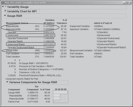
The report shown in Exhibit 8.27 appears (the script is saved as Gauge R&R). In the Gauge R&R panel, the entry for Gauge R&R under the column Measurement Source indicates that the MFI measurement system is taking up 7.32 units, which is 122 percent of the tolerance range. This is clearly indicative of a poor measurement system—its variability range exceeds the tolerance range!
Furthermore, both the repeatability and reproducibility variation are quite large and similar in magnitude, with repeatability variation using 5.13 units of the tolerance range and reproducibility variation using 5.23 units. The largest contributors to reproducibility variation are Instrument (3.99 units) and Instrument interacting with Batch, denoted Instrument*Batch (2.67 units). The analysis indicates that both the repeatability and reproducibility variation must be addressed and that team members should concentrate on variation connected with Instrument when they address reproducibility.
Figure 8.27. Gauge R&R Report for Initial MFI MSA
A variance component is an estimate of a variance. The primary variance components of interest are given in the Variance Components for Gauge R&R panel, where Carl finds estimates of the variance in MFI values due to:
Repeatability: Repeated measurements of the same part by the same operator with the same instrument.
Reproducibility: Repeated measurements of the same part by different operators using different instruments.
Part-to-Part: Differences in the parts used in the MSA; here parts are represented by batches.
Note that the variance components for Repeatability and Reproducibility sum to the variance component for Gauge R&R, which is an estimate of the measurement process variance. The total variance is the sum of the Gauge R&R variance component and the Part-to-Part variance component. In an MSA, we are typically not directly interested in part-to-part variation. In fact, we often intentionally choose parts that represent a range of variability.
The bar graph in the Variance Components for Gauge R&R panel shows that the Gauge R&R variance component is very large compared to the Part-to-Part variance component. This suggests that the measurement system has difficulty distinguishing batches. Also, the bar graph indicates that the repeatability and reproducibility variances, where Instrument variation is included in the latter, are essentially of equal magnitude, again pointing out that both must be addressed.
8.4.2. MSA for Xf
Next, the team enlists technicians in conducting an MSA for Xf. The test that measures Xf, called the ash test, measures the concentration of filler in the final polymer as a percent of total weight. The Xf value reported for a given batch is the mean of two or three ash measurements per batch. Adjustments are made to the next batch based on the results of a test on the previous batch. The ash measurement involves taking a sample of polymer, weighing it, heating it in an oven to remove all the organic material, then weighing the remaining inorganic content, which is virtually all filler. The ratio of the filler weight to the initial weight is the reported result and reflects the concentration of filler.
This is a relatively time-consuming test that takes about one hour per sample. So, it is imperative that this is taken into consideration when designing the study. Also, like the test for MFI, the ash test is a destructive test, meaning that repeated measurements will not be true replicates. However, as in the MSA for MFI, a sample will be collected from the batch and divided into aliquots; these aliquots will be considered similar enough to form a basis for repeatability estimates.
A single dedicated oven is used for the test. Three instruments are available within the laboratory to perform the weight measurements, and there are six different technicians who do the testing. The team decides that an MSA involving all six technicians would be too time-consuming, so three of the technicians are randomly chosen to participate. A study is designed using samples from 3 randomly chosen batches of polymer. These will be measured on each of the 3 instruments by each of the 3 technicians. Again, 2 repetitions of each measurement will be taken.
This results in a total of 54 tests, with each technician performing 18 tests. At an hour per test, this will take each technician about 18 hours in total; however, the technicians can complete other work while the samples are in the oven. The laboratory manager agrees that this is an acceptable amount of time. The constraint on the duration of the study is the oven, which can be used for only one sample at a time. So, a two-week period is designated for the study, with the intent that Xf samples will be worked in between other ash tests performed as part of the laboratory's regular work. The Xf study is completely randomized. As mentioned earlier, to come as close to true repeated measurements as possible, a single sample is taken from each of the three batches of polymer, and the resulting sample is divided into the 18 required aliquots.
The study is conducted, and the design and results are given in MSA_Xf_Initial.jmp. The first thing that the team wants to see is a variability chart. As before, Carl selects Graph > Variability/Gauge Chart, and enters: Xf as Y,Response; Operator then Instrument as X,Grouping; and Batch as Part,Sample ID. He clicks OK. From the red triangle, he again chooses Connect Cell Means, Show Group Means, and Show Grand Mean, and deselects Std Dev Chart. He obtains the graph shown in Exhibit 8.28 and saves the script as Variability Chart.
Figure 8.28. Variability Chart for Initial Xf MSA

The team members observe that given the variability in readings it is impossible to differentiate the batches. For example, a team member points out that measurements made by one of the technicians, Eduardo, using Instrument B do not distinguish the three batches. Repeatability variation seems large as well. Consider Eduardo's two measurements of Batch 2 using Instrument C—they appear to differ by about 2.5 units. Moreover, it appears that measurements made with Instrument A are systematically lower than those made with the other two instruments.
Carl proceeds to obtain a gauge R&R analysis. From the red triangle in the variability chart report, he chooses Gauge Studies > Gauge RR. He clicks OK to accept the Crossed default in the model type menu. Again, there is a short wait before the next dialog box appears. Since no tolerance interval has been specified for Xf, when the Enter/Verify Gauge R&R Specifications dialog opens, Carl simply clicks OK. The report in Exhibit 8.29 appears. He saves the script as Gauge R&R.
Since no tolerance range for Xf has ever been determined, the key to whether Xf is being measured with enough precision is determined by whether it can distinguish different batches, in this case the three batches that were used for the study. (Carl realizes that in the production setting two or three measurements are typically taken, which increases precision. But his intent in this MSA is to estimate the precision of a single measurement.)
Carl focuses on the Variance Components for Gauge R&R report. He notes that the Gauge R&R variance component is much larger than the Part-to-Part variance component. As was the case for MFI, this is indicative of a measurement system in trouble. Carl notes that the reproducibility and repeatability variance components are large and comparable in size.
Turning his attention to the Gauge R&R report, Carl studies the column Variation (6*StdDev), which gives variation in units of percent ash. The ranges of percent ash units taken up by repeatability and reproducibility variation are quite similar, 3.89 percent and 3.92 percent, respectively. However, what stands out immediately is that Instrument is by far the largest source of reproducibility variation, taking up 3.50 percent ash units. It is clear that the two main issues to be dealt with are the repeatability and the Instrument reproducibility, which in this case involves three scales.
Figure 8.29. Gauge R&R Report for Initial Xf MSA

8.4.3. Setting a New Timeline and Fixing the Measurement Systems
The findings from the MSAs for MFI and Xf deal a major blow to the project timetable. But Carl and his team realize that they cannot proceed until these measurement issues are resolved. Furthermore, based on the results of the MSAs, the team determines that the historical data obtained by the crisis team are largely useless. Carl's team will need to collect new data. The team estimates that in total this will cause at least a three-month delay to the project—six weeks to sort out the measurement issues and then another six weeks to obtain enough new data to analyze.
Carl explains the situation to his sponsor. After the initial shock, Edward is very supportive. "So, that means that we have been flying blind for the last ten years. But at least it explains why we have never been able to resolve this issue. Go get some good data and let's see what it tells us!"
With this guidance, Carl and his team enlist the help of the technicians and engineers who know the measurement processes for MFI and Xf. Together they begin work on improving the measurement systems.
Fixing the MFI measurement process requires the team to address the root causes of the high repeatability variation, reproducibility variation due to instrument, and variation due to the instrument and batch interaction. Observation of the process reveals that after being removed from the slurry tank, samples can sit for different lengths of time waiting to be analyzed. Also, processing steps can occur in various orders and experience time delays. It is suspected that this is a major cause of the repeatability variation. After careful study, a standard operating procedure is developed specifying the sequence of operations and timeline to be followed in processing the samples.
The other issue, reproducibility, revolves around the four melt flow meters. Here, a quick examination of the four meters in use shows that two of them are older units, and that the dies are quite worn. This could account for the differences in how the instruments measure overall as well as for batch-specific differences, which are quantified in the Instrument*Batch interaction. As part of the improvement strategy, these two units are replaced with new units, and the set of four is tested and calibrated to ensure consistent readings.
Analysis of the measurement process for Xf by the team and technicians also revealed two key issues whose root causes need to be addressed. The first of these is oven control. Sometimes technicians have other tasks that make it difficult to wait until the oven has reached its target temperature or to leave the sample in for the prescribed length of time. This explains the repeatability issues that surfaced in the MSA.
A two-part solution is proposed and approved. First, an oven probe, with a portable remote monitor capable of broadcasting alerts, is purchased. In addition, work assignments are reorganized so that a technician is always in the area of the oven when a test is being run.
The second issue relates to the instrument reproducibility problem. The team learns that the scales that are being used to weigh the filler are archaic analog scales. They are replaced by high-precision digital scales. Finally, to control other sources of variation, standardized operating procedures for testing Xf are developed and implemented with the help of the technicians.
8.4.4. Follow-up MSAs for MFI and Xf
After implementing these improvements to both measurement systems, Carl's team designs follow-up measurement system studies.
The follow-up MSA for MFI has the same structure as did the initial study. The results are given in the table MSA_MFI_Final.jmp. The variability chart is shown in Exhibit 8.30, and the Gauge R&R results are given in Exhibit 8.31. Carl saves the scripts and names them Variability Chart and Gauge R&R, respectively.
The team members and technicians look at the variability chart and are delighted! Compared to the variability among the three batches, there is very little repeatability or reproducibility variation evident.
Figure 8.30. Variability Chart for Follow-Up MFI MSA

Figure 8.31. Gauge R&R Report for Follow-Up MFI MSA
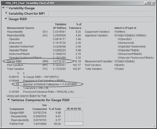
Carl notes that the Gauge R&R value given in the Gauge R&R panel is 0.61. This means that the measurement system only takes up about 0.61 units, which is almost exactly 10 percent of the tolerance range (recall that the specification limits are 192 and 198). The measurement system is now sufficiently accurate in classifying batches as good or bad relative to the specification limits on MFI. Also, the measurement system is doing well relative to the variation in batches—Carl notes that the Number of Distinct Categories value is 14.
As for Xf, the follow-up MSA is conducted with the three technicians who were not part of the original study. The results are given in MSA_Xf_Final.jmp. The variability chart is shown in Exhibit 8.32, and the Gauge R&R results are shown in Exhibit 8.33. Again, Carl has saved the scripts as Variability Chart and Gauge R&R, respectively.
Figure 8.32. Variability Chart for Follow-Up Xf MSA
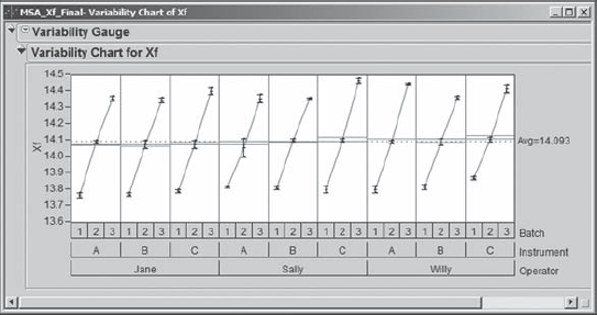
Figure 8.33. Gauge R&R Report for Follow-Up Xf MSA

Once again, the team members and technicians are pleased. Compared to the variability among the three batches, there is little repeatability or reproducibility variation.
The Gauge R&R value given in the Gauge R&R panel is 0.199 units, while the Part Variation, referring to batches in this case, is 1.168. Although these three batches were randomly selected, Carl acknowledges that they may not provide a good estimate of process variability. He notes that it would make sense to obtain a control-chart-based estimate of process variability for future comparisons.
All the same, Carl examines the Precision to Part Variation, which is 0.199/1.168 = 0.170, shown near the bottom of the Gauge R&R panel. This indicates that the measurement system is reasonably efficient at distinguishing batches based on Xf measurements. The team had hoped that this ratio would be 10 percent or less, but 17 percent is quite respectable. Also, the Number of Distinct Categories is 8, which is usually considered adequate. (In fact, based on this analysis, the decision was made to stop the practice of measuring two or more samples from each batch.)
To ensure that both the MFI and Xf measurement systems continue to operate at their current levels, measurement control systems are introduced in the form of periodic checks, monthly calibration, semiannual training, and annual MSAs.