9.6. Modeling Relationships: Recursive Partitioning

Mi-Ling turns her attention to the JMP partition platform, which implements a version of classification and regression tree analysis.^[] The partition platform allows both the response and predictors to be either continuous or categorical. Continuous predictors are split into two partitions according to cutting values, while predictors that are nominal or ordinal are split into two groups of levels. Intuitively, the split is chosen so as to maximize the difference in response between the two branches, or nodes, resulting from the split.

If the response is continuous, the sum of squares due to the difference between means is a measure of the difference in the two groups. Both the variable to be split and the cutting value for the split are determined by maximizing a quantity, called the LogWorth, which is related to the p-value associated with the sum of squares due to the difference between means. In the case of a continuous response, the fitted values are the means within the two groups.

If the response is categorical, as in Mi-Ling's case, the splits are determined by maximizing a LogWorth statistic that is related to the p-value of the likelihood ratio chi-square statistic, which is referred to as G^2. In this case, the fitted values are the estimated proportions, or response rates, within the resulting two groups.

Mi-Ling remembers hearing that the partition platform is useful both for exploring relationships and for modeling: It is very flexible, allowing a user to find not only splits that are optimal in a global sense, but also node-specific splits that satisfy various criteria. The platform provides a simple stopping rule—that is, a criterion to end splitting—based on a user-defined minimum node size. This is advantageous in that it allows flexibility at the discretion of the user.

To fit her partition model, Mi-Ling selects Analyze > Modeling > Partition. She enters Diagnosis as Y, Response and the Thirty Predictors grouping consisting of all 30 predictor variables as X, Factor. When she clicks OK, she sees the initial report shown in Exhibit 9.83. The initial node is shown, indicating under Count that there are 347 rows of data. The bar graph in the node and the plot above the node use the color red to indicate malignant values (red triangles) and blue to indicate benign values (blue circles).

Figure 9.83. Initial Partition Report

Mi-Ling would like JMP to display the proportions of malignant and benign records in each node, so she selects Display Options > Show Split Prob from the red triangle at the top of the report. When she clicks on this, the diagram updates to show the split proportions in the initial node, and will show these in all subsequent nodes as well.

Now the report appears as shown in Exhibit 9.84. Mi-Ling sees that the benign proportion is 0.6369 and the malignant proportion is 0.3631. She infers that the horizontal line separating the benign points from the malignant points in the plot at the top of the report is at about 0.64. Mi-Ling saves the script for this analysis as Initial Partition Report Window.

Figure 9.84. Initial Partition Report with Split Probabilities

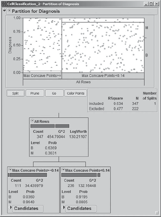
Now, Mi-Ling begins to split by clicking once on the Split button. JMP determines the best variable on which to split and the best cutting value for that variable.

The tree, after the first split, is shown in Exhibit 9.85. The first split is on the variable Max Concave Points, and the observations are split at the value where Max Concave Points = 0.14. Of the 111 observations where Max Concave Points ≥ 0.14 (the leftmost node), 96.40 percent are malignant. Of the 236 for which Max Concave Points < 0.14, 91.95 percent are benign. Mi-Ling notices that the graph at the top updates to incorporate the information about the first split, suggesting that the first split has done very well in discriminating between benign and malignant tumors.

Figure 9.85. Partition Report after First Split

Mi-Ling continues to split for a total of eight splits (Exhibit 9.86). At this point, she notices that no further splits occur. After a little thinking and a call to James, she realizes that splitting stops because JMP has set a minimum split size. In the drop-down menu obtained by clicking on the red triangle at the top of the report, Mi-Ling finds Minimum Size Split. By selecting this, she discovers that the minimum split size is set at five by default. She realizes that she could have set a larger Minimum Size Split value, which would have stopped the splitting earlier. In fact, she may have overfit the data, given that some of the final nodes contain very few observations. All the same, she decides that she will consider the eight-split model. (You might like to explore models obtained using larger values of Minimum Size Split.)

Figure 9.86. Partition Tree after Eight Splits

Mi-Ling notices that there are many options available from the red triangle menu at the top of the report, including Leaf Report, Column Contributions, K-Fold Cross Validation, ROC Curve, Lift Curve, and so on. She has used ROC and lift curves before. They are used to assess model fit. For this model, Mi-Ling plans to assess model fit by computing the misclassification rate, as she did with her logistic fits. For reasons of space, we will not discuss these additional options. We do encourage you to explore these using the documentation in Help.

A Small Tree View that condenses the information in the large tree is provided as shown in Exhibit 9.87. This small schematic shows the split variables and the split values in the tree. Mi-Ling notices that the eight splits resulted in nine terminal nodes, that is, nodes where no further splitting occurs. The splits occurred on Max Concave Points, Max Perimeter, Max Radius, Mean Texture, SE Area, SE Symmetry, and Max Texture. So, concavity, area, texture, and symmetry variables are involved.

Figure 9.87. Small Tree View for Partition Model

Mi-Ling saves her report as the script Partition Model. She is now ready to save the prediction equation to the data table. From the red triangle at the top of the report, she chooses Save Columns > Save Prediction Formula. She sees that this saves two new columns to the data table, Prob(Diagnosis==B) and Prob(Diagnosis==M).

By clicking on the plus sign to the right of Prob(Diagnosis==M) in the columns panel, Mi-Ling is able to view its formula, shown in Exhibit 9.88. She sees that this formula has the effect of placing a new observation into a terminal node based on its values on the split variables, and then assigning to that new observation a probability of malignancy equal to the proportion of malignant outcomes observed for training data records in that node. It follows that the classification rule consists of determining the terminal node into which a new observation falls and classifying it into the class with the higher sample proportion in that node.

Figure 9.88. Formula for Prob(Diagnosis==M)

To define the classification rule, Mi-Ling creates a new column called Partition Prediction. She constructs a formula to define this column; this formula classifies an observation as M if Prob(Diagnosis==M) >= 0.5, B if Prob(Diagnosis==M) < 0.5, and missing otherwise. Mi-Ling's formula is shown in Exhibit 9.89. (Alternatively, you may run the script Partition Prediction to create this column from the saved probability columns.)

Figure 9.89. Formula for Partition Prediction

She then returns to Analyze > Fit Y by X, and enters Partition Prediction as Y, Response, and Diagnosis as X, Factor. The resulting mosaic plot and contingency table are shown in Exhibit 9.90. Of the 347 rows, 11 are misclassified. At first blush, this model does not seem to be performing as well as the logistic model, which had only five misclassifications in the training set. In a later section, Mi-Ling will compare this model to the logistic model by evaluating it on the validation data set. She saves the script as Contingency – Partition Model.

Figure 9.90. Contingency Report for Partition Model Classification