CHAPTER
8

Searching for Data

Structuring your data, indexing it efficiently, and being able to perform more complex searches over it is a serious challenge. As the size of your data set grows from gigabytes to terabytes, it becomes increasingly difficult to find the data you are looking for efficiently. Any time you read, update, delete, or even insert new data, your applications and data stores need to perform searches to be able to locate the right rows (or data structures) that need to be read and written. To be able to understand better how to search through billions of records efficiently, you first need to get familiar with how indexes work.

Introduction to Indexing

Being able to index data efficiently is a critical skill when working with scalable websites. Even if you do not intend to be an expert in this field, you need to have a basic understanding of how indexes and searching work to be able to work with ever-growing data sets.

Let’s consider an example to explain how indexes and searching work. Let’s say that you had personal data of a billion users and you needed to search through it quickly (I use a billion records to make scalability issues more apparent here, but you will face similar problems on smaller data sets as well). If the data set contained first names, last names, e-mail addresses, gender, date of birth, and an account number (user ID), in such a case your data could look similar to Table 8-1.

Table 8-1 Sample of Test User Data Set

If your data was not indexed in any way, you would not be able to quickly find users based on any criteria. The only way to find a user would be to scan the entire data set, row by row. If you had a billion users and wanted to check if a particular e-mail address was in your database, you would need to perform up to a billion comparisons. In the worst-case scenario, when a user was not in your data set, you would need to perform one billion comparisons (as you cannot be sure that user is not there until you check all of the rows). It would also take you, on average, half a billion comparisons to find a user that exists in your database, because some users would live closer to the beginning and others closer to the end of the data set.

A full table scan is often the term used for this type of search, as you need to scan the entire data set to find the row that you are looking for. As you can imagine, that type of search is expensive. You need to load all of the data from disk into memory to be able to perform comparisons and check if the row at hand is the one you are looking for. A full table scan is pretty much the worst-case scenario when it comes to searching, as it has O(n) cost.

Because a full table scan has a linear cost, it is not an efficient way to search large data sets. A common way to speed up searching is to create an index on the data that you are going to search upon. For example, if you wanted to search for users based on their e-mail address, you would create an index on the e-mail address field.

In a simplified way, you can think of an index as a lookup data structure, just like a book index. To build a book index, you sort terms (keywords) in alphabetic order and map each of them to a page number. When readers want to find pages referring to a particular term, they can quickly locate the term in the index and find page numbers that they should look at. Figure 8-1 shows how data is structured in a book index.

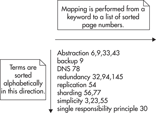
Figure 8-1 Book index structure

There are two important properties of an index:

   An index is structured and sorted in a specific way, optimized for particular types of searches. For example, a book index can answer questions like “What pages refer to the term sharding?” but it cannot answer questions like “What pages refer to more than one term?” Although both questions refer to locations of terms in the book, a book index is not optimized to answer the second question efficiently.

   The data set is reduced in size because the index is much smaller in size than the overall body of text so that the index can be loaded and processed faster. A 400-page book may have an index of just a few pages. That makes searching for terms faster, as there is less content to search through.

The reason why most indexes are sorted is that searching through a sorted data set can be performed much faster than through an unsorted one. A good example of a simple and fast searching algorithm is the binary search algorithm. When using a binary search algorithm, you don’t scan the data set from the beginning to the end, but you “jump around,” skipping large numbers of items. The algorithm takes a range of sorted values and performs four simple steps until the value is found:

1. You look at the middle item of the data set to see if the value is equal, greater to, or smaller than what you are searching for.

2. If the value is equal, you found the item you were looking for.

3. If the value is greater than what you are looking for, you continue searching through the smaller items. You go back to step 1 with the data set reduced by half.

4. If the value is smaller than what you are looking for, you continue searching through the larger items. You go back to step 1 with the data set reduced by half.

Figure 8-2 shows how binary search works on a sequence of sorted numbers. As you can see, you did not have to investigate all of the numbers.

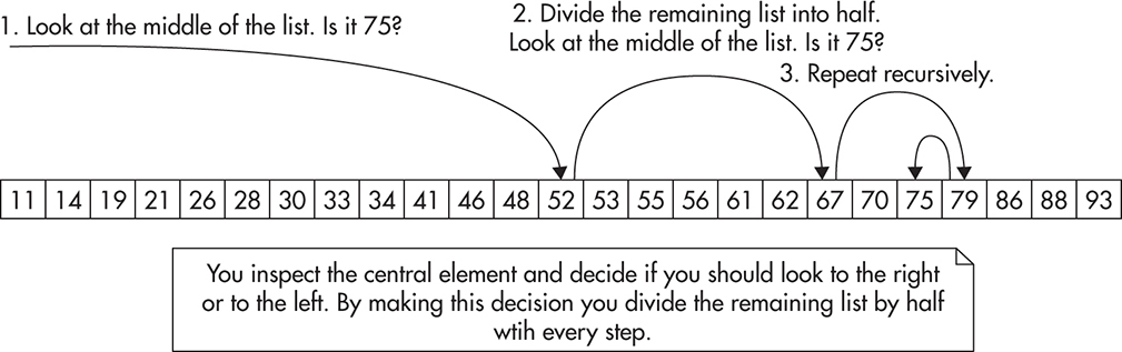
Figure 8-2 Searching for number 75 using binary search

The brilliance of searching using this method is that with every comparison you reduce the number of items left by half. This in turn allows you to narrow down your search rapidly. If you had a billion user IDs, you would only need to perform, on average, 30 comparisons to find what you are looking for! If you remember, a full table scan would take, on average, half a billion comparisons to locate a row. The binary search algorithm has a Big O notation cost of O(log2n), which is much lower than the O(n) cost of a full table scan.

It is worth getting familiar with Big O notation, as applying the right algorithms and data structures becomes more important as your data set grows. Some of the most common Big O notation expressions are O(n^2), (n*log(n)), O(n), O(log(n)), and O(1). Figure 8-3 shows a comparison of these curves, with the horizontal axis being the data set size and the vertical axis showing the relative computation cost. As you can see, the computational complexity of O(n^2) grows very rapidly, causing even small data sets to become an issue. On the other hand, O(log(n)) grows so slowly that you can barely notice it on the graph. In comparison to the other curves, O(log(n)) looks more like a constant time O(1) than anything else, making it very effective for large data sets.

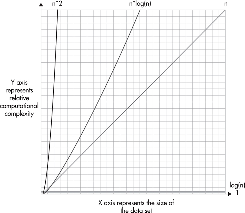
Figure 8-3 Big O notation curves

Indexes are great for searching, but unfortunately, they add some overhead. Maintaining indexes requires you to keep additional data structures with sorted lists of items, and as the data set grows, these data structures can become large and costly. In this example, indexing 1 billion user IDs could grow to a monstrous 16GB of data. Assuming that you used 64-bit integers, you would need to store 8 bytes for the user ID and 8 bytes for the data offset for every single user. At such scale, adding indexes needs to be well thought out and planned, as having too many indexes can cost you a great amount of memory and I/O (the data stored in the index needs to be read from the disk and written to it as well).

To make it even more expensive, indexing text fields like e-mail addresses takes more space because the data being indexed is “longer” than 8 bytes. On average, e-mail addresses are around 20 bytes long, making indexes even larger.

Considering that indexes add overhead, it is important to know what data is worth indexing and what is not. To make these decisions, you need to look at the queries that you intend to perform on your data and the cardinality of each field.

To explain better how to estimate cardinality, let’s take a look at the example data set again. The following are all of the fields with estimated cardinality:

   gender In most databases, there would be only two genders available, giving us very low cardinality (cardinality ~ 2). Although you can find databases with more genders (like transsexual male), the overall cardinality would still be very low (a few dozen at best).

   date of birth Assuming that your users were mostly under 80 years old and over 10 years old, you end up with up to 25,000 unique dates (cardinality ~ 25000). Although 25,000 dates seems like a lot, you will still end up with tens or hundreds of thousands of users born on each day, assuming that distribution of users is not equal and you have more 20-year-old users than 70-year-old ones.

   first name Depending on the mixture of origins, you might have tens of thousands of unique first names (cardinality ~ tens of thousands).

   last name This is similar to first names (cardinality ~ tens of thousands).

   email address If e-mail addresses were used to uniquely identify accounts in your system, you would have cardinality equal to the total number of rows (cardinality = 1 billion). Even if you did not enforce e-mail address uniqueness, they would have few duplicates, giving you a very high cardinality.

   user id Since user IDs are unique, the cardinality would also be 1 billion (cardinality = 1 billion).

The reason why low-cardinality fields are bad candidates for indexes is that they do not narrow down the search enough. After traversing the index, you still have a lot of rows left to inspect. Figure 8-4 shows two indexes visualized as sorted lists. The first index contains user IDs and the location of each row in the data set. The second index contains the gender of each user and reference to the data set.

Figure 8-4 Field cardinality and index efficiency

Both of the indexes shown in Figure 8-4 are sorted and optimized for different types of searches. Index A is optimized to search for users based on their user ID, and index B is optimized to search for users based on their gender.

The key point here is that searching for a match on the indexed field is fast, as you can skip large numbers of rows, just as the binary search algorithm does. As soon as you find a match, though, you can no longer narrow down the search efficiently. All you can do is inspect all remaining rows, one by one. In this example, when you find a match using index A, you get a single item; in comparison, when you find a match using index B, you get half a billion items.

HINT

The first rule of thumb when creating indexes on a data set is that the higher the cardinality, the better the index performance.

The cardinality of a field is not the only thing that affects index performance. Another important factor is the item distribution. If you were indexing a field where some values were present in just a single item and others were present in millions of records, then performance of the index would vary greatly depending on which value you look for. For example, if you indexed a date of birth field, you are likely going to end up with a bell curve distribution of users. You may have a single user born on October 4, 1923, and a million users born on October 4, 1993. In this case, searching for users born on October 4, 1923, will narrow down the search to a single row. Searching for users born on October 4, 1993, will result in a million items left to inspect and process, making the index less efficient.

HINT

The second rule of thumb when creating indexes is that equal distribution leads to better index performance.

Luckily, indexing a single field and ending up with a million items is not the only thing you can do. Even when cardinality or distribution of values on a single field is not great, you can create indexes that have more than one field, allowing you to use the second field to narrow down your search further.

If you use compound indexes, in addition to deciding which fields to index, you need to decide in what order they should be indexed. When you create a compound index, you effectively create a sorted list ordered by multiple columns. It is just as if you sorted data by multiple columns in Excel or Google Docs. Depending on the order of columns in the compound index, the sorting of data changes. Figure 8-5 shows two indexes: index A (indexing first name, last name, and date of birth) and index B (indexing last name, first name, and date of birth).

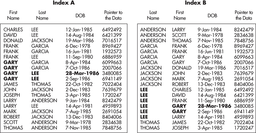
Figure 8-5 Ordering of columns in a compound index

The most important thing to understand here is that indexes A and B are optimized for different types of queries. They are similar, but they are not equal, and you need to know exactly what types of searches you are going to perform to choose which one is better for your application.

Using index A, you can efficiently answer the following queries:

   get all users where first name = Gary

   get all users where first name = Gary and last name = Lee

   get all users where first name = Gary and last name = Lee and date of birth = March 28, 1986

Using index B, you can efficiently answer the following queries:

   get all users where last name = Lee

   get all users where last name = Lee and first name = Gary

   get all users where last name = Lee and first name = Gary and date of birth = March 28, 1986

As you might have noticed, queries 2 and 3 in both cases can be executed efficiently using either one of the indexes. The order of matching values would be different in each case, but it would result in the same number of rows being found and both indexes would likely have comparable performance.

To make it more interesting, although both indexes A and B contain date of birth, it is impossible to efficiently search for users born on April 8, 1984, without knowing their first and last names. To be able to search through index A, you need to have a first name that you want to look for. Similarly, if you want to search through index B, you need to have the user’s last name. Only when you know the exact value of the leftmost column can you narrow down your search by providing additional information for the second and third columns.

Understanding the indexing basics presented in this section is absolutely critical to being able to design and implement scalable web applications. In particular, if you want to use NoSQL data stores, you need to stop thinking of data as if it were stored in tables and think of it as if it were stored in indexes. Let’s explore this idea in more detail and see how you can optimize your data model for fast access despite large data size.

Modeling Data

When you use NoSQL data stores, you need to get used to thinking of data as if it were an index.

The main challenge when designing and building the data layer of a scalable web application is identifying access patterns and modeling your data based on these access patterns. Data normalization and simple rules of thumb learned from relational databases are not enough when working with terabytes of data. Huge data sets and the technical limitations of data stores will force you to design your data model much more carefully and consider use cases over the data relationships.

To be able to scale your data layer, you need to analyze your access patterns and use cases, select a data store, and then design the data model. To make it more challenging, you need to keep the data model as flexible as possible to allow for future extensions. At the same time, you want to optimize it for fast access to keep up with the growth of the data size.

These two forces often conflict, as optimizing the data model usually reduces the flexibility; conversely, increasing flexibility often leads to worse performance and scalability. In the following subsections we will discuss some NoSQL modeling techniques and concrete NoSQL data model examples to better explain how it is done in practice and what tradeoffs you need to prepare yourself for. Let’s start by looking at NoSQL data modeling.

NoSQL Data Modeling

If you used relational databases before, you are likely familiar with the process of data modeling. When designing a relational database schema, you would usually start by looking at the data itself. You would ask yourself, “What is the data that I need to store?” You would then go through all of the bits of information that need to be persisted and isolate entities (database tables). You would then decide which pieces of information should be stored in which table. You would also create relationships between tables using foreign keys. You would then iterate over the schema design, trying to reduce the amount of redundant data and circular relationships.

As a result of this process, you would usually end up with a normalized and flexible database schema that could be used to answer almost any type of question using SQL queries. You would usually finish this process without thinking much about particular features or what feature would need to execute what types of queries. Your schema would be designed mainly based on the data itself, not queries or use cases. Later on, as you implement your application and new types of queries are needed, you would create new indexes to speed up these queries, but the data schema would usually remain unchanged, as it would be flexible enough to handle any type of query.

Unfortunately, that process of design and normalization focused on data does not work when applied to NoSQL data stores. NoSQL data stores trade data model flexibility (and ability to perform joins) for scalability, so you need to find a different approach.

To be able to model data in NoSQL data stores and access it efficiently, you need to change the way you design your schema. Rather than starting with data in mind, you need to start with queries in mind. I would argue that designing a data model in the NoSQL world is more difficult than it is in the relational database world. Once you optimize your data model for particular types of queries, you usually lose the ability to perform other types of queries. Designing a NoSQL data model is much more about tradeoffs and data layout optimization than it is about normalization.

When designing a data model for a NoSQL data store, you want to identify all the queries and access patterns first. Only once you understand how your data will be accessed can you move on to identifying key pieces of data and looking for ways to structure it so that you could execute all of your query types efficiently.

For example, if you were designing an e-commerce website using a relational database, you might not think much about how data would be queried. You might decide to have separate tables for products, product categories, and product reviews. Figure 8-6 shows how your data model might look.

Figure 8-6 Relational data model

If you were designing the same type of e-commerce website and you had to support millions of products with millions of user actions per hour, you might decide to use a NoSQL data store to help you scale the system. You would then have to model your data around your main queries rather than using a generic normalized model.

For example, if your most important queries were to load a product page to display all of the product-related metadata like name, image URL, price, categories it belongs to, and average user ranking, you might optimize your data model for this use case rather than keeping it normalized. Figure 8-7 shows an alternative data model with example documents in each of the collections.

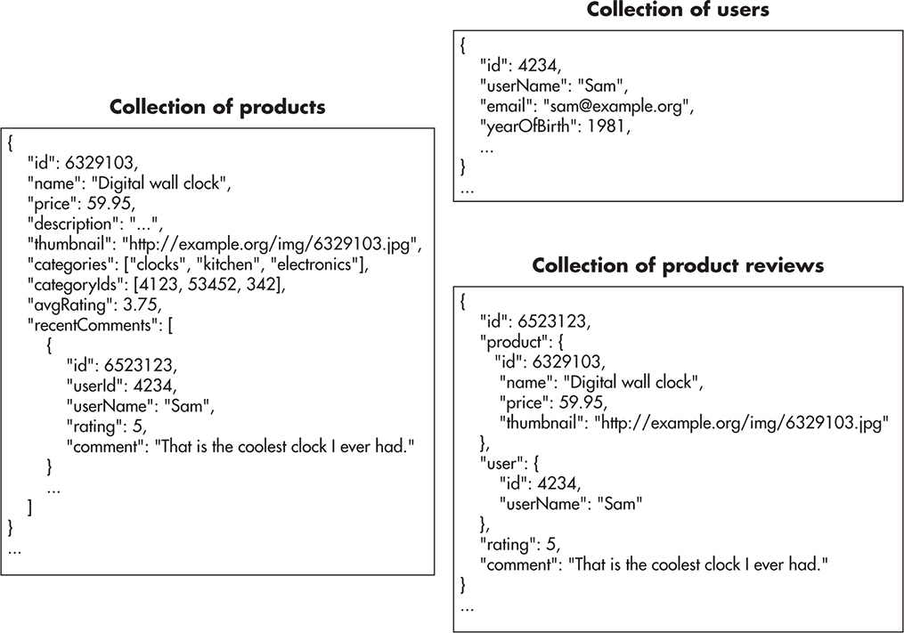
Figure 8-7 Nonrelational data model

By grouping most of the data into the product entity, you would be able to request all of that data with a single document access. You would not need to join tables, query multiple servers, or traverse multiple indexes. Rendering a product page could then be achieved by a single index lookup and fetching of a single document. Depending on the data store used, you might also shard data based on the product ID so that queries regarding different products could be sent to different servers, increasing your overall capacity.

There are considerable benefits and drawbacks of data denormalization and modeling with queries in mind. Your main benefit is performance and ability to efficiently access data despite a huge data set. By using a single index and a single “table,” you minimize the number of disk operations, reducing the I/O pressure, which is usually the main bottleneck in the data layer.

On the other hand, denormalization introduces data redundancy. In this example, in the normalized model (with SQL tables), category names live in a separate table and each product is joined to its categories by a product_categories table. This way, category metadata is stored once and product metadata is stored once (product_categories contains references only). In the denormalized approach (NoSQL-like), each product has a list of category names embedded. Categories do not exist by themselves—they are part of product metadata. That leads to data redundancy and, what is more important here, makes updating data much more difficult. If you needed to change a product category name, you would need to update all of the products that belong to that category, as category names are stored within each product. That could be extremely costly, especially if you did not have an index allowing you to find all products belonging to a particular category. In such a scenario, you would need to perform a full table scan and inspect all of the products just to update a category name.

HINT

Flexibility is one of the most important attributes of good architecture. To quote Robert C. Martin again, “Good architecture maximizes the number of decisions not made.” By denormalizing data and optimizing for certain access patterns, you are making a tradeoff. You sacrifice some flexibility for the sake of performance and scalability. It is critical to be aware of these tradeoffs and make them very carefully.

As you can see, denormalization is a double-edged sword. It helps us optimize and scale, but it can be restricting and it can make future changes much more difficult. It can also easily lead to a situation where there is no efficient way to search for data and you need to perform costly full table scans. It can also lead to situations where you need to build additional “tables” and add even more redundancy to be able to access data efficiently.

Regardless of the drawbacks, data modeling focused on access patterns and use cases is what you need to get used to if you decide to use NoSQL data stores. As mentioned in Chapter 5, NoSQL data stores are more specialized than relational database engines and they require different data models. In general, NoSQL data stores do not support joins and data has to be grouped and indexed based on the access patterns rather than based on the meaning of the data itself.

Although NoSQL data stores are evolving very fast and there are dozens of open-source projects out there, the most commonly used NoSQL data stores can be broadly categorized based on their data model into three categories:

   Key-value data stores These data stores support only the most simplistic access patterns. To access data, you need to provide the key under which data was stored. Key-value stores have a limited programming interface—basically all you can do is set or get objects based on their key. Key-value stores usually do not support any indexes or sorting (other than the primary key). At the same time, they have the least complexity and they can implement automatic sharding based on the key, as each value is independent and the only way to access values is by providing their keys. They are good for fast one-to-one lookups, but they are impractical when you need sorted lists of objects or when you need to model relationships between objects. Examples of key-value stores are Dynamo and Riak. Memcached is also a form of a key-value data store, but it does not persist data, which makes it more of a key-value cache than a data store. Another data store that is sometimes used as a key-value store is Redis, but it has more to offer than just key-value mappings.

   Wide columnar data stores These data stores allow you to model data as if it was a compound index. Data modeling is still a challenge, as it is quite different from relational databases, but it is much more practical because you can build sorted lists. There is no concept of a join, so denormalization is a standard practice, but in return wide columnar stores scale very well. They usually provide data partitioning and horizontal scalability out of the box. They are a good choice for huge data sets like user-generated content, event streams, and sensory data. Examples of wide columnar data stores are BigTable, Cassandra, and HBase.

   Document-oriented data stores These data stores allow more complex objects to be stored and indexed by the data store. Document-based data stores use a concept of a document as the most basic building block in their data model. Documents are data structures that can contain arrays, maps, and nested structures just as a JSON or XML document would. Although documents have flexible schemas (you can add and remove fields at will on a per-document basis), document data stores usually allow for more complex indexes to be added to collections of documents. Document stores usually offer a fairly rich data model, and they are a good use case for systems where data is difficult to fit into a predefined schema (where it is hard to create a SQL-like normalized model) and at the same time where scalability is required. Examples of document-oriented data stores are MongoDB, CouchDB, and Couchbase.

There are other types of NoSQL data stores like graph databases and object stores, but they are still much less popular. Going into more detail about each of these data store types is outside the scope of this book, especially because the NoSQL data store market is very fragmented, with each of the data stores evolving in a slightly different direction to satisfy specialized niche needs.

Instead of trying to cover all of the possible data stores, let’s have a look at a couple of data model examples to see how NoSQL modeling works in practice.

Wide Column Storage Example

Consider an example where you needed to build an online auction website similar in concept to eBay. If you were to design the data model using the relational database approach, you would begin by looking for entities and normalize the model. As I mentioned before, in the NoSQL world, you need to start by looking at what queries you are going to perform, not just what data you are going to store.

Let’s say that you had the following list of use cases that need to be satisfied:

1. Users need to be able to sign up and log in.

2. Logged-in users can view auction details by viewing the item auction page.

3. The item auction page contains product information like title, description, and images.

4. The item auction page also includes a list of bids with the names of users who placed them and the prices they offered.

5. Users need to be able to change their user name.

6. Users can view the history of bids of other users by viewing their profile pages. The user profile page contains details about the user like name and reputation score.

7. The user profile page shows a list of items that the user placed bids on. Each bid displays the name of the item, a link to the item auction page, and a price that the user offered.

8. Your system needs to support hundreds of millions of users and tens of millions of products with millions of bids each.

After looking at the use cases, you might decide to use a wide columnar data store like Cassandra. By using Cassandra, you can leverage its high availability and automated horizontal scalability. You just need to find a good way to model these use cases to make sure that you can satisfy the business needs.

The Cassandra data model is often represented as a table with an unlimited number of rows and a nearly unlimited number of arbitrary columns, where each row can have different columns, and column names can be made up on the spot (there is no table definition or strict schema and columns are dynamically created as you add fields to the row). Figure 8-8 shows how the Cassandra table is usually illustrated.

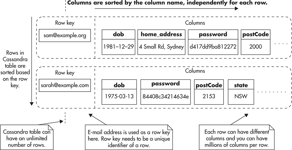
Figure 8-8 Fragments of two rows in a Cassandra table

Each row has a row key, which is a primary key and at the same time a sharding key of the table. The row key is a string—it uniquely identifies a single row and it is automatically indexed by Cassandra. Rows are distributed among different servers based on the row key, so all of the data that needs to be accessed together in a single read needs to be stored within a single row. Figure 8-8 also shows that rows are indexed based on the row key and columns are indexed based on a column name.

The way Cassandra organizes and sorts data in tables is similar to the way compound indexes work. Any time you want to access data, you need to provide a row key and then column name, as both of these are indexed. Because columns are stored in sorted order, you can perform fast scans on column names to retrieve neighboring columns. Since every row lives on its own and there is no table schema definition, there is no way to efficiently select multiple rows based on a particular column value.

You could visualize a Cassandra table as if it was a compound index. Figure 8-9 shows how you could define this model in a relational database like MySQL. The index would contain a row key as the first field and then column name as the second field. Values would contain actual values from Cassandra fields so that you would not need to load data from another location.

Figure 8-9 Cassandra table represented as if it were a compound index

As I mentioned before, indexes are optimized for access based on the fields that are indexed. When you want to access data based on a row key and a column name, Cassandra can locate the data quickly, as it traverses an index and does not need to perform any table scans. The problem with this approach is that queries that do not look for a particular row key and column may be inefficient because they require expensive scans.

HINT

Many NoSQL data modeling techniques can be boiled down to building compound indexes so that data can be located efficiently. As a result, queries that can use the index perform very well, but queries that do not use the index require a full table scan.

Going back to the example of an online auction website, you could model users in Cassandra by creating a users table. You could use the user’s e-mail address (or user name) as a row key of the users table so that you could find users efficiently when they are logging in to the system. To make sure you always have the user’s row key, you could then store it in the user’s HTTP session or encrypted cookies for the duration of the visit.

You would then store user attributes like first name, last name, phone number, and hashed password in separate columns of the users table. Since there is no predefined column schema in Cassandra, some users might have additional columns like billing address, shipping address, or contact preference settings.

HINT

Any time you want to query the users table, you should do it for a particular user to avoid expensive table scans. As I mentioned before, Cassandra tables behave like compound indexes. The row key is the first field of that “index,” so you always need to provide it to be able to search for data efficiently. You can also provide column names or column name ranges to find individual attributes. The column name is the second field of the “compound index” and providing it improves search speed even further.

In a similar way, you could model auction items. Each item would be uniquely identified by a row key as its ID. Columns would represent item attributes like title, image URLs, description, and classification. Figure 8-10 shows how both the users table and items table might look. By having these two tables, you can efficiently find any item or user by their row key.

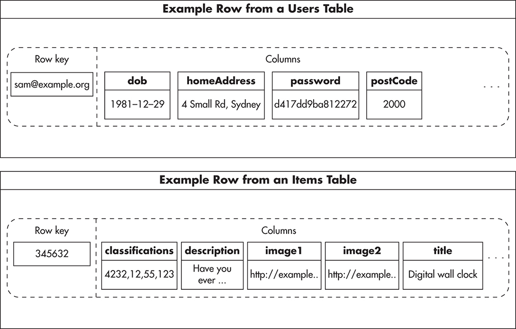
Figure 8-10 User and item tables

To satisfy more use cases, you would also need to store information about which users placed bids on which items. To be able to execute all of these queries efficiently, you would need to store this information in a way that is optimized for two access patterns:

   Get all bids of a particular item (use case 4)

   Get all bids of a particular user (use case 7)

To allow these access patterns, you need to create two additional “indexes”: one indexing bids by item ID and the second one indexing bids by user ID. As of this writing Cassandra does not allow you to index selected columns, so you need to create two additional Cassandra tables to provide these indexes. You could create one table called item_bids to store bids per item and a second table called user_bids to store bids per user.

Alternatively, you could use another feature of Cassandra called column families to avoid creating additional tables. By using column families, you would still end up with denormalized and duplicated data, so for simplicity’s sake I decided to use separate tables in this example. Any time a user places a bid, your web application needs to write to both of these data structures to keep both of these “indexes” in sync. Luckily, Cassandra is optimized for writes and writing to multiple tables is not a concern from a scalability or performance point of view.

Figure 8-11 shows how these two tables might look. If you take a closer look at the user_bids table, you may notice that column names contain timestamps and item IDs. By using this trick, you can store bids sorted by time and display them on the user’s profile page in chronological order.

Figure 8-11 Tables storing bids based on item and user

By storing data in this way you are able to write into these tables very efficiently. Any time you need to place a bid, you would serialize bid data and simply issue two commands:

   set data under column named “$time|$item_id” for a row “$user_email” in table user_bids

   set data under column named “$time|$user_email” for a row “$item_id” in table item_bids

Cassandra is an eventually consistent store, so issuing writes this way ensures that you never miss any writes. Even if some writes are delayed, they still end up in the same order on all servers. No matter how long it takes for such a command to reach each server, data is always inserted into the right place and stored in the same order. In addition, order of command execution on each server becomes irrelevant, and you can issue the same command multiple times without affecting the end result (making these commands idempotent).

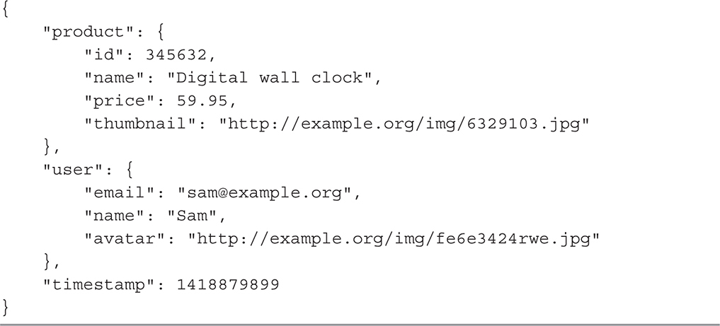
It is also worth noting here that bid data would be denormalized and redundant, as shown in Listing 8-1. You would set the same data in both user_bids and item_bids tables. Serialized bid data would contain enough information about the product and the bidding user so that you would not need to fetch additional values from other tables to render bids on the user’s profile page or item detail pages. This data demineralization would allow you to render an item page with a single query on the item table and a single column scan on the item_bids table. In a similar way, you could render the user’s profile page by a single query to the users table and a single column scan on the user_bids table.

Listing 8-1 Serialized bid data stored in column values

Once you think your data model is complete, it is critical to validate it against the list of known use cases. This way, you can ensure that your data model can, in fact, support all of the access patterns necessary. In this example, you could go over the following use cases:

   To create an account and log in (use case 1), you would use e-mail address as a row key to locate the user’s row efficiently. In the same way, you could detect whether an account for a given e-mail address exists or not.

   Loading the item auction page (use cases 2, 3, and 4) would be performed by looking up the item by ID and then loading the most recent bids from the item_bids table. Cassandra allows fetching multiple columns starting from any selected column name, so bids could be loaded in chronological order. Each item bid contains all the data needed to render the page fragment and no further queries are necessary.

   Loading the user page (use cases 6 and 7) would work in a similar way. You would fetch user metadata from the users table based on the e-mail address and then fetch the most recent bids from the user_bids table.

   Updating the user name is an interesting use case (use case 5), as user names are stored in all of their bids in both user_bids and item_bids tables. Updating the user name would have to be an offline process because it requires much more data manipulation. Any time a user decides to update his or her user name, you would need to add a job to a queue and defer execution to an offline process. You would be able to find all of the bids made by the user using the user_bids table. You would then need to load each of these bids, unserialize them, change the embedded user name, and save them back. By loading each bid from the user_bids table, you would also find its timestamp and item ID. That, in turn, would allow you to issue an additional SET command to overwrite the same bid metadata in the item_bids table.

   Storing billions of bids, hundreds of millions of users, and millions of items (user case 8) would be possible because of Cassandra’s auto-sharding functionality and careful selection of row keys. By using user ID and an item ID as row keys, you are able to partition data into small chunks and distribute it evenly among a large number of servers. No auction item would receive more than a million bids and no user would have more than thousands or hundreds of thousands of bids. This way, data could be partitioned and distributed efficiently among as many servers as was necessary.

There are a few more tradeoffs that are worth pointing out here. By structuring data in a form of a “compound index,” you gain the ability to answer certain types of queries very quickly. By denormalizing the bid’s data, you gain performance and help scalability. By serializing all the bid data and saving it as a single value, you avoid joins, as all the data needed to render bid page fragments are present in the serialized bid object.

On the other hand, denormalization of a bid’s data makes it much more difficult and time consuming to make changes to redundant data. By structuring data as if it were an index, you optimize for certain types of queries. This, in turn, makes some types of queries perform exceptionally well, but all others become prohibitively inefficient.

Finding a flexible data model that supports all known access patterns and provides maximal flexibility is the real challenge of NoSQL. For example, using the data model presented in this example, you cannot efficiently find items with the highest number of bids or the highest price. There is no “index” that would allow you to efficiently find this data, so you would need to perform a full table scan to get these answers. To make things worse, there is no easy way to add an index to a Cassandra table. You would need to denormalize it further by adding new columns or tables.

An alternative way to deal with the NoSQL indexing challenge is to use a dedicated search engine for more complex queries rather than trying to satisfy all use cases with a single data store. Let’s now have a quick look at search engines and see how they can complement a data layer of a scalable web application.

Search Engines

Nearly every web application needs to perform complex search queries nowadays. For example, e-commerce platforms need to allow users to search for products based on arbitrary combinations of criteria like category, price range, brand, availability, or location. To make things even more difficult, users can also search for arbitrary words or phrases and apply sorting according to their own preferences.

Whether you use relational databases or NoSQL data stores, searching through large data sets with such flexibility is going to be a significant challenge even if you apply the best modeling practices and use the best technologies available on the market.

Allowing users to perform such wide ranges of queries requires either building dozens of indexes optimized for different types of searches or using a dedicated search engine. Before deciding whether you need a dedicated search engine, let’s start with a quick introduction to search engines to understand better what they do and how they do it.

Introduction to Search Engines

You can think of search engines as data stores specializing in searching through text and other data types. As a result, they make different types of tradeoffs than relational databases or NoSQL data stores do. For example, consistency and write performance may be much less important to them than being able to perform complex searches very fast. They may also have different needs when it comes to memory consumption and I/O throughput as they optimize for specific interaction patterns.

Before you begin using dedicated search engines, it is worth understanding how full text search works itself. The core concept behind full text search and modern search engines is an inverted index.

The types of indexes that we discussed so far required you to search for an exact value match or for a value prefix. For example, if you built an index on a text field containing movie titles, you could efficiently find rows with a title equal to “It’s a Wonderful Life.” Some index types would also allow you to efficiently search for all titles starting with a prefix “It’s a Wonderful,” but they would not let you search for individual words in a text field. If your user typed in “Wonderful Life,” he or she would not find the “It’s a Wonderful Life” record unless you used a full text search (an inverted index). Using an inverted index allows you to search for any of the words contained in the text field, regardless of their location and order. For example, you could search for “Life Wonderful” or “It’s a Life” and still find the “It’s a Wonderful Life” record.

When you index a piece of text like “The Silence of the Lambs” using an inverted index, it is first broken down into tokens (like words). Then each of the tokens can be preprocessed to improve search performance. For example, all words may be lowercased, plural forms changed to singular, and duplicates removed from the list. As a result, you may end up with a smaller list of unique tokens like “the,” “silence,” “of,” “lamb.”

Once you extract all the tokens, you then use them as if they were keywords in a book index. Rather than adding a movie title in its entirety into the index, you add each word independently with a pointer to the document that contained it. Figure 8-12 shows the structure of a simplistic inverted index.

Figure 8-12 Inverted index structure

As shown in Figure 8-12, document IDs next to each token are in sorted order to allow a fast search within a list and, more importantly, merging of lists. Any time you want to find documents containing particular words, you first find these words in the dictionary and then merge their posting lists.

HINT

The structure of an inverted index looks just like a book index. It is a sorted list of words (tokens) and each word points to a sorted list of page numbers (document IDs).

Searching for a phrase (“silence” AND “lamb”) requires you to merge posting lists of these two words by finding an intersection. Searching for words (“silence” OR “lamb”) requires you to merge two lists by finding a union. In both cases, merging can be performed efficiently because lists of document IDs are stored in sorted order. Searching for phrases (AND queries) is slightly less expensive, as you can skip more document IDs and the resulting merged list is usually shorter than in the case of OR queries. In both cases, though, searching is still expensive and carries an O(n) time complexity (where n is the length of posting lists).

Understanding how an inverted index works may help to understand why OR conditions are especially expensive in a full text search and why search engines need so much memory to operate. With millions of documents, each containing thousands of words, an inverted index grows in size faster than a normal index would because each word in each document must be indexed.

Understanding how different types of indexes work will also help you design more efficient NoSQL data models, as NoSQL data modeling is closer to designing indexes than designing relational schemas. In fact, Cassandra was initially used at Facebook to implement an inverted index and allow searching through the messages inbox.^w27 Having said that, I would not recommend implementing a full text search engine from scratch, as it would be very expensive. Instead, I would recommend using a general-purpose search engine as an additional piece of your infrastructure. Let’s have a quick look at a common search engine integration pattern.

Using a Dedicated Search Engine

As I mentioned before, search engines are data stores specializing in searching. They are especially good at full text searching, but they also allow you to index other data types and perform complex search queries efficiently. Any time you need to build a rich search functionality over a large data set, you should consider using a search engine.

A good place to see how complex searching features can become is to look at used car listings websites. Some of these websites have hundreds of thousands of cars for sale at a time, which forces them to provide much more advanced searching criteria (otherwise, users would be flooded with irrelevant offers). As a result, you can find advanced search forms with literally dozens of fields. You can search for anything from free text, mark, model, min/max price, min/max mileage, fuel type, transmission type, horsepower, and color to accessories like electric mirrors and heated seats. To make things even more complicated, once you execute your search, you want to display facets to users to allow them to narrow down their search even further by selecting additional filters rather than having to start from scratch.

Complex search functionality like this is where dedicated search engines really shine. Rather than having to implement complex and inefficient solutions yourself in your application, you are much better off by using a search engine. There are a few popular search engines out there: search engines as a service, like Amazon CloudSearch and Azure Search, and open-source products, like Elasticsearch, Solr, and Sphinx.

If you decide to use a hosted service, you benefit significantly from not having to operate, scale, and manage these components yourself. Search engines, especially the cutting-edge ones, can be quite difficult to scale and operate in production, unless you have engineers experienced with this particular technology. You may sacrifice some flexibility and some of the edge-case features, but you reduce your time to market and the complexity of your operations.

Going into the details of how to configure, scale, and operate search engines is beyond the scope of this book, but let’s have a quick look at how you could integrate with one of them. For example, if you decided to use Elasticsearch as a search engine for your used car sales website, you would need to deploy it in your data center and index all of your cars in it. Indexing cars using Elasticsearch would be quite simple since Elasticsearch does not require any predefined schema. You would simply need to generate JSON documents for each car and post them to be indexed by Elasticsearch. In addition, to keep the search index in sync with your primary data store, you would need to refresh the documents indexed in Elasticsearch any time car metadata changes.

HINT

A common pattern for indexing data in a search engine is to use a job queue (especially since search engines are near real time anyway). Anytime anyone modifies car metadata, they submit an asynchronous message for this particular car to be reindexed. At a later stage, a queue worker picks up the message from the queue, builds up the JSON document with all the information, and posts to the search engine to overwrite previous data.

Figure 8-13 shows how a search engine deployment could look. All of the searches would be executed by the search engine. Search results could then be enriched by real-time data coming from the main data store (if it was absolutely necessary). On the other hand, people editing their car listings would write directly to the main data store and refresh the search index via a queue and an asynchronous indexing worker process.

Figure 8-13 Inverted index structure

By having all of your cars indexed by Elasticsearch, you could then start issuing complex queries like “Get all cars mentioning ‘quick sale’ made by Toyota between 2000 and 2005 with electric windows and tagged as special offer. Then sort it all by price and product facets like location, model, and color.”

Search engines are an important tool in the NoSQL web stack toolbelt, and I strongly recommend getting familiar with at least a couple of platforms to be able to choose and use them efficiently.

Summary

Being able to search for data efficiently can be a serious challenge. The key things to take away from this chapter are that data should be stored in a way that is optimized for specific access patterns and that indexes are the primary tool for making search scalable.

It is also important to remember that NoSQL brings a new way of thinking about data. You identify your main use cases and access patterns and derive the data model out of this knowledge rather than structuring data in a generic way. It may also require dedicated search engines, to complement your infrastructure and deal with the most complex search scenarios.

Explore searching, indexing, and data modeling in more detail.^{16,19,w27–w28,w47–w48,w71} Searching for data was the last purely technical chapter of this book; let’s now have a look at some other dimensions of scalability in the context of web startups.