

This chapter discusses the memory hierarchy — the different types and performance levels of memory found in computer systems. Although programmers often treat all forms of memory as though they were equivalent, using memory improperly can have a negative impact on performance. This chapter discusses how to make the best use of the memory hierarchy within your programs.
Most modern programs benefit by having a large amount of very fast memory. Unfortunately, as a memory device gets larger, it tends to be slower. For example, cache memories are very fast, but they are also small and expensive. Main memory is inexpensive and large, but is slow, requiring wait states. The memory hierarchy provides a way to compare the cost and performance of memory. Figure 11-1 diagrams one variant of the memory hierarchy.
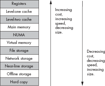
At the top level of the memory hierarchy are the CPU’s general-purpose registers. The registers provide the fastest access to data possible on the CPU. The register file is also the smallest memory object in the hierarchy (for example, the 80x86 has just eight general-purpose registers). Because it is impossible to add more registers to a CPU, registers are also the most expensive memory locations. Even if we count the FPU, MMX/AltaVec, SSE/SIMD, and other CPU registers in this portion of the memory hierarchy, this does not change the fact that CPUs have a very limited number of registers, and the cost per byte of register memory is quite high.
Working our way down, the level-one cache system is the next highest performance subsystem in the memory hierarchy. As with registers, the CPU manufacturer usually provides the level-one (L1) cache on the chip, and you cannot expand it. The size is usually small, typically between 4 KB and 32 KB, though this is much larger than the register memory available on the CPU chip. Although the L1 cache size is fixed on the CPU, the cost per cache byte is much lower than the cost per register byte because the cache contains more storage than is available in all the combined registers, and the system designer’s cost of both memory types is the price of the CPU.
Level-two cache is present on some CPUs, but not all. For example, most Pentium II, III, and IV CPUs have a level-two (L2) cache as part of the CPU package, but some of Intel’s Celeron chips do not. The L2 cache is generally much larger than the L1 cache (for example, 256 KB to 1 MB as compared with 4 KB to 32 KB). On CPUs with a built-in L2 cache, the cache is not expandable. It is still lower in cost than the L1 cache because we amortize the cost of the CPU across all the bytes in the two caches, and the L2 cache is larger.
The main-memory subsystem comes below the L2 cache system in the memory hierarchy.[43] Main memory is the general-purpose, relatively low-cost memory found in most computer systems. Typically, this memory is DRAM or some similarly inexpensive memory. However, there are many differences in main memory technology that result in differences in speed. The main memory types include standard DRAM, synchronous DRAM (SDRAM), double data rate DRAM (DDRAM), and Rambus DRAM (RDRAM). Generally, though, you won’t find a mixture of these technologies in the same computer system.
Below main memory is the NUMA memory subsystem. NUMA, which stands for Non-Uniform Memory Access, is a bit of a misnomer. The term NUMA implies that different types of memory have different access times, and so it is descriptive of the entire memory hierarchy. In Figure 11-1, however, the term NUMA is used to describe blocks of memory that are electronically similar to main memory but, for one reason or another, operate significantly slower than main memory. A good example of NUMA memory is the memory on a video display card. Another example is flash memory, which has significantly slower access and transfer times than standard semiconductor RAM. Other peripheral devices that provide a block of memory to be shared between the CPU and the peripheral usually have slow access times, as well.
Most modern computer systems implement a virtual memory scheme that simulates main memory using a mass storage disk drive. A virtual memory subsystem is responsible for transparently copying data between the disk and main memory as needed by programs. While disks are significantly slower than main memory, the cost per bit is also three orders of magnitude lower for disks. Therefore, it is far less expensive to keep data on magnetic storage than in main memory.
File storage also uses disk media to store program data. However, whereas the virtual memory subsystem is responsible for handling data transfer between disk and main memory as programs require, it is the program’s responsibility to store and retrieve file-storage data. In many instances, it is a bit slower to use file-storage memory than it is to use virtual memory, hence the lower position of file-storage memory in the memory hierarchy.[44]
Next comes network storage. At this level in the memory hierarchy, programs keep data on a different memory system that connects to the computer system via a network. Network storage can be virtual memory, file-storage memory, or a memory system known as distributed shared memory (DSM), where processes running on different computer systems share data stored in a common block of memory and communicate changes to that block across the network.
Virtual memory, file storage, and network storage are examples of so-called online memory subsystems. Memory access within these memory subsystems is slower than accessing the main-memory subsystem. However, when a program requests data from one of these three memory subsystems, the memory device will respond to the request as quickly as its hardware allows. This is not true for the remaining levels in the memory hierarchy.
The near-line and offline storage subsystems may not be ready to respond to a program’s request for data immediately. An offline storage system keeps its data in electronic form (usually magnetic or optical), but on storage media that are not necessarily connected to the computer system that needs the data. Examples of offline storage include magnetic tapes, disk cartridges, optical disks, and floppy diskettes. Tapes and removable media are among the most inexpensive electronic data storage formats available. Hence, these media are great for storing large amounts of data for long periods. When a program needs data from an offline medium, the program must stop and wait for someone or something to mount the appropriate media on the computer system. This delay can be quite long (perhaps the computer operator decided to take a coffee break?).
Near-line storage uses the same types of media as offline storage, but rather than requiring an external source to mount the media before its data is available for access, the near-line storage system holds the media in a special robotic jukebox device that can automatically mount the desired media when a program requests it.
Hard-copy storage is simply a printout, in one form or another, of data. If a program requests some data, and that data is present only in hard-copy form, someone will have to manually enter the data into the computer. Paper, or other hard-copy media, is probably the least expensive form of memory, at least for certain data types.
The whole point of having the memory hierarchy is to allow reasonably fast access to a large amount of memory. If only a little memory were necessary, we’d use fast static RAM (the circuitry that cache memory uses) for everything. If speed wasn’t an issue, we’d use virtual memory for everything. The whole point of having a memory hierarchy is to enable us to take advantage of the principles of spatial locality of reference and temporality of reference to move often-referenced data into fast memory and leave less-often-used data in slower memory. Unfortunately, during the course of a program’s execution, the sets of oft-used and seldom-used data change. We cannot simply distribute our data throughout the various levels of the memory hierarchy when the program starts and then leave the data alone as the program executes. Instead, the different memory subsystems need to be able to adjust for changes in spatial locality or temporality of reference during the program’s execution by dynamically moving data between subsystems.
Moving data between the registers and memory is strictly a program function. The program loads data into registers and stores register data into memory using machine instructions like mov. It is strictly the programmer’s or compiler’s responsibility to keep heavily referenced data in the registers as long as possible, the CPU will not automatically place data in general-purpose registers in order to achieve higher performance.
Programs are largely unaware of the memory hierarchy between the register level and main memory. In fact, programs only explicitly control access to registers, main memory, and those memory-hierarchy subsystems at the file-storage level and below. In particular, cache access and virtual memory operations are generally transparent to the program. That is, access to these levels of the memory hierarchy usually occurs without any intervention on a program’s part. Programs simply access main memory, and the hardware and operating system take care of the rest.
Of course, if every memory access that a program makes is to main memory, then the program will run slowly because modern DRAM main-memory subsystems are much slower than the CPU. The job of the cache memory subsystems and of the CPU’s cache controller is to move data between main memory and the L1 and L2 caches so that the CPU can quickly access oft-requested data. Likewise, it is the virtual memory sub-system’s responsibility to move oft-requested data from hard disk to main memory (if even faster access is needed, the caching subsystem will then move the data from main memory to cache).
With few exceptions, most memory subsystem accesses take place transparently between one level of the memory hierarchy and the level immediately below or above it. For example, the CPU rarely accesses main memory directly. Instead, when the CPU requests data from memory, the L1 cache subsystem takes over. If the requested data is in the cache, then the L1 cache subsystem returns the data to the CPU, and that concludes the memory access. If the requested data is not present in the L1 cache, then the L1 cache subsystem passes the request on down to the L2 cache subsystem. If the L2 cache subsystem has the data, it returns this data to the L1 cache, which then returns the data to the CPU. Note that requests for the same data in the near future will be fulfilled by the L1 cache rather than the L2 cache because the L1 cache now has a copy of the data.
If neither the L1 nor the L2 cache subsystems have a copy of the data, then the request goes to main memory. If the data is found in main memory, then the main-memory subsystem passes this data to the L2 cache, which then passes it to the L1 cache, which then passes it to the CPU. Once again, the data is now in the L1 cache, so any requests for this data in the near future will be fulfilled by the L1 cache.
If the data is not present in main memory, but is present in virtual memory on some storage device, the operating system takes over, reads the data from disk or some other device (such as a network storage server), and passes the data to the main-memory subsystem. Main memory then passes the data through the caches to the CPU in the manner that we’ve seen.
Because of spatial locality and temporality, the largest percentage of memory accesses take place in the L1 cache subsystem. The next largest percentage of accesses takes place in the L2 cache subsystem. The most infrequent accesses take place in virtual memory.
If you take another look at Figure 11-1, you’ll notice that the speed of the various memory hierarchy levels increases as you go up. Exactly how much faster is each successive level in the memory hierarchy? To summarize the answer here, the speed gradient is not uniform. The speed difference between any two contiguous levels ranges from “almost no difference” to “four orders of magnitude.”
Registers are, unquestionably, the best place to store data you need to access quickly. Accessing a register never requires any extra time, and most machine instructions that access data can access register data. Furthermore, instructions that access memory often require extra bytes (displacement bytes) as part of the instruction encoding. This makes instructions longer and, often, slower.
If you read Intel’s instruction timing tables for the 80x86, you’ll see that they claim that an instruction like mov(someVar,ecx); is supposed to run as fast as an instruction of the form mov(ebx,ecx);. However, if you read the fine print, you’ll find that they make this claim based on several assumptions about the former instruction. First, they assume that someVar’s value is present in the L1 cache memory. If it is not, then the cache controller needs to look in the L2 cache, in main memory, or worse, on disk in the virtual memory subsystem. All of a sudden, an instruction that should execute in one nano-second on a 1-GHz processor (that is, in one clock cycle) requires several milliseconds to execute. That’s a difference of over six orders of magnitude. It is true that future accesses of this variable will take place in just one clock cycle because it will subsequently be stored in the L1 cache. But even if you access someVar’s value one million times while it is still in the cache, the average time of each access will still be about two cycles because of the large amount of time needed to access someVar the very first time.
Granted, the likelihood that some variable will be located on disk in the virtual memory subsystem is quite low. However, there is still a difference in performance of three orders of magnitude between the L1 cache subsystem and the main memory subsystem. Therefore, if the program has to bring the data from main memory, 999 memory accesses later you’re still paying an average cost of two clock cycles to access the data that Intel’s documentation claims should happen in one cycle.
The difference in speed between the L1 and L2 cache systems is not so dramatic unless the secondary cache is not packaged together on the CPU. On a 1-GHz processor the L1 cache must respond within one nanosecond if the cache operates with zero wait states (some processors actually introduce wait states in L1 cache accesses, but CPU designers try to avoid this). Accessing data in the L2 cache is always slower than in the L1 cache, and there is always the equivalent of at least one wait state, and up to eight, when accessing data in the L2 cache.
There are several reasons why L2 cache accesses are slower than L1 accesses. First, it takes the CPU time to determine that the data it is seeking is not in the L1 cache. By the time it determines that the data is not present in the L1 cache, the memory-access cycle is nearly complete, and there is no time to access the data in the L2 cache. Secondly, the circuitry of the L2 cache may be slower than the circuitry of the L1 cache in order to make the L2 cache less expensive. Third, L2 caches are usually 16 to 64 times larger than L1 caches, and larger memory subsystems tend to be slower than smaller ones. All this adds up to additional wait states when accessing data in the L2 cache. As noted earlier, the L2 cache can be as much as one order of magnitude slower than the L1 cache.
The L1 and L2 caches also differ in the amount of data the system fetches when there is a cache miss (see Chapter 6). When the CPU fetches data from or writes data to the L1 cache, it generally fetches or writes only the data requested. If you execute a mov(al,memory); instruction, the CPU writes only a single byte to the cache. Likewise, if you execute the mov(mem32,eax); instruction, the CPU reads exactly 32 bits from the L1 cache. However, access to memory subsystems below the L1 cache does not work in small chunks like this. Usually, memory subsystems move blocks of data, or cache lines, whenever accessing lower levels of the memory hierarchy. For example, if you execute the mov(mem32,eax); instruction, and mem32’s value is not in the L1 cache, the cache controller doesn’t simply read mem32’s 32 bits from the L2 cache, assuming that it’s present there. Instead, the cache controller will actually read a whole block of bytes (generally 16, 32, or 64 bytes, depending on the particular processor) from the L2 cache. The hope is that the program exhibits spatial locality and therefore that reading a block of bytes will speed up future accesses to adjacent objects in memory. The bad news, however, is that the mov(mem32,eax); instruction doesn’t complete until the L1 cache reads the entire cache line from the L2 cache. This excess time is known as latency. If the program does not access memory objects adjacent to mem32 in the future, this latency is lost time.
A similar performance gulf separates the L2 cache and main memory. Main memory is typically one order of magnitude slower than the L2 cache. To speed up access to adjacent memory objects, the L2 cache reads data from main memory in blocks (cache lines) to speed up access to adjacent memory elements.
Standard DRAM is three to four orders of magnitude faster than disk storage. To overcome this difference, there is usually a difference of two to three orders of magnitude in size between the L2 cache and the main memory so that the difference in speed between disk and main memory matches the difference in speed between the main memory and the L2 cache. (Having balanced performance characteristics is an attribute to strive for in the memory hierarchy in order to effectively use the different memory levels.)
We will not consider the performance of the other memory-hierarchy subsystems in this chapter, as they are more or less under programmer control. Because their access is not automatic, very little can be said about how frequently a program will access them. However, in Chapter 12 we’ll take another look at issues regarding these storage devices.
Up to this point, we have treated the cache as a magical place that automatically stores data when we need it, perhaps fetching new data as the CPU requires it. But how exactly does the cache do this? And what happens when the cache is full and the CPU is requesting additional data not in the cache? In this section, we’ll look at the internal cache organization and try to answer these questions, along with a few others.
Because programs only access a small amount of data at a given time, a cache that is the same size as the typical amount of data that programs access can provide very high-speed data access. Unfortunately, the data that programs want rarely sits in contiguous memory locations. Usually the data is spread out all over the address space. Therefore, cache design has to accommodate the fact that the cache must map data objects at widely varying addresses in memory.
As noted in the previous section, cache memory is not organized in a single group of bytes. Instead, cache memory is usually organized in blocks of cache lines, with each line containing some number of bytes (typically a small power of two like 16, 32, or 64), as shown in Figure 11-2.
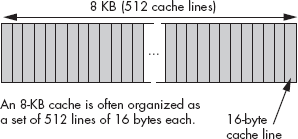
Because of this 512×16-byte cache organization found in Figure 11-2, we can attach a different noncontiguous address to each of the cache lines. Cache line 0 might correspond to addresses $10000..$1000F and cache line 1 might correspond to addresses $21400..$2140F. Generally, if a cache line is n bytes long, that cache line will hold n bytes from main memory that fall on an n-byte boundary. In the example in Figure 11-2, the cache lines are 16 bytes long, so a cache line holds blocks of 16 bytes whose addresses fall on 16-byte boundaries in main memory (in other words, the LO four bits of the address of the first byte in the cache line are always zero).
When the cache controller reads a cache line from a lower level in the memory hierarchy, where does the data go in the cache? The answer is determined by the caching scheme in use. There are three different cache schemes: direct-mapped cache, fully associative cache, and n-way set associative cache.
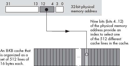
In a direct-mapped cache (also known as the one-way set associative cache), a block of main memory is always loaded into the exact same cache line. Generally, a small number of bits in the data’s memory address determines which cache line will hold the data. For example, Figure 11-3 shows how the cache controller could select the appropriate cache line for an 8-KB cache with 512 16-byte cache lines and a 32-bit main-memory address. Because there are 512 cache lines, it requires 9 bits to select one of the cache lines (29 = 512). This example uses bits 4 through 12 to determine which cache line to use (assuming we number the cache lines from 0 to 511), while bits 0 through 3 of the original memory address determine the particular byte within the 16-byte cache line.
The direct-mapped cache scheme is very easy to implement. Extracting nine (or some other number of) bits from the memory address and using the result as an index into the array of cache lines is trivial and fast. However, direct-mapped caches suffer from a few problems.
Perhaps the biggest problem with a direct-mapped cache is that it may not make effective use of all the cache memory. For example, the cache scheme in Figure 11-3 maps address zero to cache line 0. It also maps addresses $2000 (8 KB), $4000 (16 KB), $6000 (24 KB), and $8000 (32 KB) to cache line 0. In fact, it maps every address that is an even multiple of eight kilobytes to cache line 0. This means that if a program is constantly accessing data at addresses that are even multiples of 8 KB and not accessing any other locations, the system will only use cache line 0, leaving all the other cache lines unused. Each time the CPU requests data at an address that is mapped to cache line 0, but whose corresponding data is not present in cache line 0 (an address that is not an even multiple of 8 KB), the CPU will have to go down to a lower level in the memory hierarchy to access the data. In this extreme case, the cache is effectively limited to the size of one cache line.
The most flexible cache system is the fully associative cache. In a fully associative cache subsystem, the caching controller can place a block of bytes in any one of the cache lines present in the cache memory. While this is a very flexible system, the flexibility required is not without cost. The extra circuitry to achieve full associativity is expensive and, worse, can slow down the memory subsystem. Most L1 and L2 caches are not fully associative for this reason.
If a fully associative cache organization is too complex, too slow, and too expensive to implement, but a direct-mapped cache organization isn’t as good as we’d like, one might ask if there is a compromise that doesn’t have the drawbacks of a direct-mapped approach or the complexity of a fully associative cache. The answer is yes; we can create an n-way set associative cache that is a compromise between these two extremes. In an n-way set associative cache, the cache is broken up into sets of cache lines. The CPU determines the particular set to use based on some subset of the memory address bits, just as in the direct-mapping scheme. Within each cache line set, there are n cache lines. The caching controller uses a fully associative mapping algorithm to determine which one of the n cache lines within the set to use.
For example, an 8-KB two-way set associative cache subsystem with 16-byte cache lines organizes the cache into 256 cache-line sets with two cache lines each. (“Two-way” means that each set contains two cache lines.) Eight bits from the memory address determine which one of these 256 different sets holds the cache line that will contain the data. Once the cache-line set is determined, the cache controller then maps the block of bytes to one of the two cache lines within the set (see Figure 11-4).
The advantage of a two-way set associative cache over a direct-mapped cache is that two different memory addresses located on 8-KB boundaries (addresses having the same value in bits 4 through 11) can both appear simultaneously in the cache. However, a conflict will occur if you attempt to access a third memory location at an address that is an even multiple of 8 KB.
A two-way set associative cache is much better than a direct-mapped cache and it is considerably less complex than a fully associative cache. However, if you’re still getting too many conflicts, you might consider using a four-way set associative cache, which puts four associative cache lines in each cache-line set. In an 8-KB cache like the one in Figure 11-4, a four-way set associative cache scheme would have 128 cache-line sets with four cache lines each. This would allow the cache to maintain up to four different blocks of data without a conflict, each of which would map to the same cache line in a direct-mapped cache.

The more cache lines we have in each cache-line set, the closer we come to creating a fully associative cache, with all the attendant problems of complexity and speed. Most cache designs are direct-mapped, two-way set associative, or four-way set associative. The various members of the 80x86 family make use of all three.
Although this chapter has made the direct-mapped cache look bad, it is, in fact, very effective for many types of data. In particular, the direct-mapped cache is very good for data that you access in a sequential rather than random fashion. Because the CPU typically executes instructions in a sequential fashion, instruction bytes can be stored very effectively in a direct-mapped cache. However, because programs tend to access data more randomly than code, a two-way or four-way set associative cache usually makes a better choice for data accesses than a direct-mapped cache.
Because data and machine instruction bytes usually have different access patterns, many CPU designers use separate caches for each. For example, a CPU designer could choose to implement an 8-KB instruction cache and an 8-KB data cache rather than a single 16-KB unified cache. The advantage of dividing the cache size in this way is that the CPU designer could use a caching scheme more appropriate to the particular values that will be stored in each cache. The drawback is that the two caches are now each half the size of a unified cache, which may cause more cache misses than would occur with a unified cache. The choice of an appropriate cache organization is a difficult one and can only be made after analyzing many running programs on the target processor. How to choose an appropriate cache format is beyond the scope of this book, but be aware that it’s not a choice you can make just by reading a textbook.
Thus far, we’ve answered the question, “Where do we put a block of data in the cache?” An equally important question we’ve ignored until now is, “What happens if a cache line isn’t available when we want to put a block of data in that cache line?”
For a direct-mapped cache architecture, the answer is trivial. The cache controller simply replaces whatever data was formerly in the cache line with the new data. Any subsequent reference to the old data will result in a cache miss, and the cache controller will then have to bring that old data back into the cache by replacing whatever data is in the appropriate cache line at that time.
For a two-way set associative cache, the replacement algorithm is a bit more complex. Whenever the CPU references a memory location, the cache controller uses some subset of the address’ bits to determine the cache-line set that should be used to store the data. Using some fancy circuitry, the caching controller determines whether the data is already present in one of the two cache lines in the destination set. If the data is not present, the CPU has to bring the data in from memory. Because the main memory data can go into either cache line, the controller has to pick one of the two lines to use. If either or both of the cache lines are currently unused, the controller simply picks an unused line. However, if both cache lines are currently in use, then the cache controller must pick one of the cache lines and replace its data with the new data.
How does the controller choose which of the two cache lines to replace? Ideally, we’d like to keep the cache line whose data will be referenced first and replace the other cache line. Unfortunately, neither the cache controller nor the CPU is omniscient — they cannot predict which of the lines is the best one to replace.
To understand how the cache controller makes this decision, remember the principle of temporality: if a memory location has been referenced recently, it is likely to be referenced again in the very near future. This implies the following corollary: if a memory location has not been accessed in a while, it is likely to be a long time before the CPU accesses it again. Therefore, a good replacement policy that many caching controllers use is the least recently used (LRU) algorithm. An LRU policy is easy to implement in a two-way set associative cache system. All you need is to reserve a single bit for each set of two cache lines. Whenever the CPU accesses one of the two cache lines this bit is set to zero, and whenever the CPU accesses the other cache line, this bit is set to one. Then, when a replacement is necessary, this bit will indicate which cache line to replace, as it tracks the last cache line the program has accessed (and, because there are only two cache lines in the set, the inverse of this bit also tracks the cache line that was least recently used).
For four-way (and greater) set associative caches, maintaining the LRU information is a bit more difficult, which is one of the reasons the circuitry for such caches is more complex. Because of the complications that LRU can introduce on these associative caches, other replacement policies are sometimes used. Two of these other policies are first-in, first-out (FIFO) and random. These are easier to implement than LRU, but they have their own problems, which are beyond the scope of this book, but which a text on computer architecture or operating systems will discuss.
What happens when the CPU writes data to memory? The simple answer, and the one that results in the quickest operation, is that the CPU writes the data to the cache. However, what happens when the cache line containing this data is subsequently replaced by data that is read from memory? If the modified contents of the cache line are not written to main memory prior to this replacement, then the data that was written to the cache line will be lost. The next time the CPU attempts to access that data it will reload the cache line with the old data that was never updated after the write operation.
Clearly any data written to the cache must ultimately be written to main memory as well. There are two common write policies that caches use: write-back and write-through. Interestingly enough, it is sometimes possible to set the write policy in software, as the write policy isn’t always hardwired into the cache controller. However, don’t get your hopes up. Generally the CPU only allows the BIOS or operating system to set the cache write policy, so unless you’re the one writing the operating system, you won’t be able to control the write policy.
The write-through policy states that any time data is written to the cache, the cache immediately turns around and writes a copy of that cache line to main memory. An important point to notice is that the CPU does not have to halt while the cache controller writes the data from cache to main memory. So unless the CPU needs to access main memory shortly after the write occurs, this writing takes place in parallel with the execution of the program. Furthermore, because the write-through policy updates main memory with the new value as rapidly as possible, it is a better policy to use when two different CPUs are communicating through shared memory.
Still, writing a cache line to memory takes some time, and it is likely that the CPU (or some CPU in a multiprocessor system) will want to access main memory during the write operation, so the write-through policy may not be a high-performance solution to the problem. Worse, suppose the CPU reads from and writes to the memory location several times in succession. With a write-through policy in place, the CPU will saturate the bus with cache-line writes, and this will have a very negative impact on the program’s performance.
The second common cache write policy is the write-back policy. In this mode, writes to the cache are not immediately written to main memory; instead, the cache controller updates main memory at a later time. This scheme tends to be higher performance because several writes to the same cache line within a short time period do not generate multiple writes to main memory.
Of course, at some point the cache controller must write the data in cache to memory. To determine which cache lines must be written back to main memory, the cache controller usually maintains a dirty bit within each cache line. The cache system sets this bit whenever it writes data to the cache. At some later time, the cache controller checks this dirty bit to determine if it must write the cache line to memory. For example, whenever the cache controller replaces a cache line with other data from memory, it must first check the dirty bit, and if that bit is set, the controller must write that cache line to memory before going through with the cache-line replacement. Note that this increases the latency time when replacing a cache line. If the cache controller were able to write dirty cache lines to main memory while no other bus access was occurring, the system could reduce this latency during cache line replacement. Some systems actually provide this functionality, and others do not for economic reasons.
A cache subsystem is not a panacea for slow memory access. In order for a cache system to be effective, software must exhibit locality of reference (either spatial or temporal). Fortunately, real-world programs tend to exhibit locality of reference, so most programs will benefit from the presence of a cache in the memory subsystem. But while programs do exhibit locality of reference, this is often accidental; programmers rarely consider the memory-access patterns of their software when designing and coding. Unfortunately, application programmers who work under the assumption that the cache will magically improve the performance of their applications are missing one important point — a cache can actually hurt the performance of an application.
Suppose that an application accesses data at several different addresses that the caching controller would map to the exact same cache line. With each access, the caching controller must read in a new cache line (possibly flushing the old cache line back to memory if it is dirty). As a result, each memory access incurs the latency cost of bringing in a cache line from main memory. This degenerate case, known as thrashing, can slow down the program by one to two orders of magnitude, depending on the speed of main memory and the size of a cache line. Great code is written with the behavior of the cache in mind. A great programmer attempts to place oft-used variables in adjacent memory cells so those variables tend to fall into the same cache lines. A great programmer carefully chooses data structures (and access patterns to those data structures) to avoid thrashing. We’ll take another look at thrashing a little later in this chapter.
Another benefit of the cache subsystem on modern 80x86 CPUs is that it automatically handles many misaligned data references. As you may recall, there is a penalty for accessing words or double-word objects at an address that is not an even multiple of that object’s size. As it turns out, by providing some fancy logic, Intel’s designers have eliminated this penalty as long as the data object is located completely within a cache line. However, if the object crosses a cache line, there will be a performance penalty for the memory access.
In a modern operating system such as Mac OS, Linux, or Windows, it is very common to have several different programs running concurrently in memory. This presents several problems.
How do you keep the programs from interfering with each other’s memory?
If one program expects to load a value into memory at address $1000, and a second program also expects to load a value into memory at address $1000, how can you load both values and execute both programs at the same time?
What happens if the computer has 64 MB of memory, and we decide to load and execute three different applications, two of which require 32 MB and one that requires 16 MB (not to mention the memory that the operating system requires for its own purposes)?
The answers to all these questions lie in the virtual memory subsystem that modern processors support.
Virtual memory on CPUs such as the 80x86 gives each process its own 32-bit address space.[45] This means that address $1000 in one program is physically different from address $1000 in a separate program. The CPU achieves this sleight of hand by mapping the virtual addresses used by programs to different physical addresses in actual memory. The virtual address and the physical address don’t have to be the same, and usually they aren’t. For example, program 1’s virtual address $1000 might actually correspond to physical address $215000, while program 2’s virtual address $1000 might correspond to physical memory address $300000. How can the CPU do this? Easy, by using paging.
The concept behind paging is quite simple. First, you break up memory into blocks of bytes called pages. A page in main memory is comparable to a cache line in a cache subsystem, although pages are usually much larger than cache lines. For example, the 80x86 CPUs use a page size of 4,096 bytes.
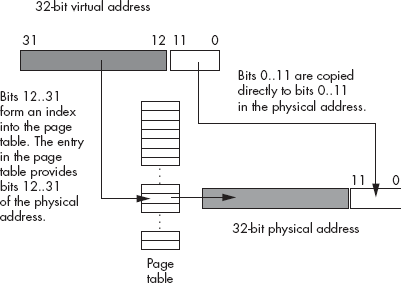
After breaking up memory into pages, you use a lookup table to map the HO bits of a virtual address to the HO bits of the physical address in memory, and you use the LO bits of the virtual address as an index into that page. For example, with a 4,096-byte page, you’d use the LO 12 bits of the virtual address as the offset (0..4095) within the page, and the upper 20 bits as an index into a lookup table that returns the actual upper 20 bits of the physical address (see Figure 11-5).
Of course, a 20-bit index into the page table would require over one million entries in the page table. If each of the over one million entries is a 32-bit value, then the page table would be 4 MB long. This would be larger than most of the programs that would run in memory! However, by using what is known as a multilevel page table, it is very easy to create a page table for most small programs that is only 8 KB long. The details are unimportant here. Just rest assured that you don’t need a 4-MB page table unless your program consumes the entire 4 GB address space.
If you study Figure 11-5 for a few moments, you’ll probably discover one problem with using a page table — it requires two separate memory accesses in order to retrieve the data stored at a single physical address in memory: one to fetch a value from the page table, and one to read from or write to the desired memory location. To prevent cluttering the data or instruction cache with page-table entries, which increases the number of cache misses for data and instruction requests, the page table uses its own cache, known as the translation lookaside buffer (TLB). This cache typically has 32 entries on a Pentium family processor — enough to handle 128 KB of memory, or 32 pages, without a miss. Because a program typically works with less data than this at any given time, most page-table accesses come from the cache rather than main memory.
As noted, each entry in the page table contains 32 bits, even though the system really only needs 20 bits to remap each virtual address to a physical address. Intel, on the 80x86, uses some of the remaining 12 bits to provide some memory-protection information:
One bit marks whether a page is read/write or read-only.
One bit determines whether you can execute code on that page.
A number of bits determine whether the application can access that page or if only the operating system can do so.
A number of bits determine if the CPU has written to the page, but hasn’t yet written to the physical memory address corresponding to the page entry (that is, whether the page is “dirty” or not, and whether the CPU has accessed the page recently).
One bit determines whether the page is actually present in physical memory or if it’s stored on secondary storage somewhere.
Note that your applications do not have access to the page table (reading and writing the page table is the operating system’s responsibility), and therefore they cannot modify these bits. However, operating systems like Windows may provide some functions you can call if you want to change certain bits in the page table (for example, Windows will allow you to set a page to read-only if you want to do so).
Beyond remapping memory so multiple programs can coexist in main memory, paging also provides a mechanism whereby the operating system can move infrequently used pages to secondary storage. Just as locality of reference applies to cache lines, it applies to pages in main memory as well. At any given time, a program will only access a small percentage of the pages in main memory that contain data and instruction bytes and this set of pages is known as the working set. Although this working set of pages varies slowly over time, for small periods of time the working set remains constant. Therefore, there is little need for the remainder of the program to consume valuable main memory storage that some other process could be using. If the operating system can save the currently unused pages to disk, the main memory they consume would be available for other programs that need it.
Of course, the problem with moving data out of main memory is that eventually the program might actually need that data. If you attempt to access a page of memory, and the page-table bit tells the memory management unit (MMU) that the page is not present in main memory, the CPU interrupts the program and passes control to the operating system. The operating system then analyzes the memory-access request and reads the corresponding page of data from the disk drive and copies it to some available page in main memory. This process is nearly identical to the process used by a fully associative cache subsystem, except that accessing the disk is much slower than accessing main memory. In fact, you can think of main memory as a fully associative write-back cache with 4,096-byte cache lines, which caches the data that is stored on the disk drive. Placement and replacement policies and other issues are very similar for caches and main memory.
However, that’s as far as we’ll go in exploring how the virtual memory subsystem works. If you’re interested in further information, any decent textbook on operating system design will explain how the virtual memory subsystem swaps pages between main memory and the disk. Our main goal here is to realize that this process takes place in operating systems like Mac OS, Linux, and Windows, and that accessing the disk is very slow.
One important issue resulting from the fact that each program has a separate page table, and the fact that programs themselves don’t have access to the page tables, is that programs cannot interfere with the operation of other programs. That is, a program cannot change its page tables in order to access data found in another process’s address space. If your program crashes by overwriting itself, it cannot crash other programs at the same time. This is a big benefit of a paging memory system.
If two programs want to cooperate and share data, they can do so by placing such data in a memory area that is shared by the two processes. All they have to do is tell the operating system that they want to share some pages of memory. The operating system returns a pointer to each process that points at a segment of memory whose physical address is the same for both processes. Under Windows, you can achieve this by using memory-mapped files; see the operating system documentation for more details. Mac OS and Linux also support memory-mapped files as well as some special shared-memory operations; again, see the OS documentation for more details.
Although this discussion applies specifically to the 80x86 CPU, multi-level paging systems are common on other CPUs as well. Page sizes tend to vary from about 1 KB to 64 KB, depending on the CPU. For CPUs that support an address space larger than 4 GB, some CPUs use an inverted page table or a three-level page table. Although the details are beyond the scope of this chapter, rest assured that the basic principle remains the same — the CPU moves data between main memory and the disk in order to keep oft-accessed data in main memory as much of the time as possible. These other page-table schemes are good at reducing the size of the page table when an application uses only a fraction of the available memory space.
Thrashing is a degenerate case that can cause the overall performance of the system to drop to the speed of a lower level in the memory hierarchy, like main memory or, worse yet, the disk drive. There are two primary causes of thrashing:
If there is insufficient memory to hold a working set of pages or cache lines, the memory system will constantly be replacing one block of data in the cache or main memory with another block of data from main memory or the disk. As a result, the system winds up operating at the speed of the slower memory in the memory hierarchy. A common example of thrashing occurs with virtual memory. A user may have several applications running at the same time, and the sum total of the memory required by these programs’ working sets is greater than all of the physical memory available to the programs. As a result, when the operating system switches between the applications it has to copy each application’s data, and possibly program instructions, to and from disk. Because switching between programs is often much faster than retrieving data from the disk, this slows the programs down by a tremendous factor.
We have already seen in this chapter that if the program does not exhibit locality of reference and the lower memory subsystems are not fully associative, then thrashing can occur even if there is free memory at the current level in the memory hierarchy. To take our earlier example, suppose an 8-KB L1 caching system uses a direct-mapped cache with 512 16-byte cache lines. If a program references data objects 8 KB apart on every access, then the system will have to replace the same line in the cache over and over again with the data from main memory. This occurs even though the other 511 cache lines are currently unused.
When insufficient memory is the problem, you can add memory to reduce thrashing. Or, if you can’t add more memory, you can try to run fewer processes concurrently or modify your program so that it references less memory over a given period. To reduce thrashing when locality of reference is causing the problem, you should restructure your program and its data structures to make its memory references physically near one another.
Although most of the RAM in a system is based on high-speed DRAM interfaced directly with the processor’s bus, not all memory is connected to the CPU in this manner. Sometimes a large block of RAM is part of a peripheral device, and you communicate with that device by writing data to its RAM. Video display cards are probably the most common example of such a peripheral, but some network interface cards, USB controllers, and other peripherals also work this way. Unfortunately, the access time to the RAM on these peripheral devices is often much slower than the access time to main memory. In this section, we’ll use the video card as an example, although NUMA performance applies to other devices and memory technologies as well.
A typical video card interfaces with a CPU via an AGP or PCI bus inside the computer system. The PCI bus typically runs at 33 MHz and is capable of transferring four bytes per bus cycle. Therefore, in burst mode, a video controller card is capable of transferring 132 MB per second, though few would ever come close to achieving this for technical reasons. Now compare this with main-memory access time. Main memory usually connects directly to the CPU’s bus, and modern CPUs have an 800-MHz 64-bit-wide bus. If memory were fast enough, the CPU’s bus could theoretically transfer 6.4 GB per second between memory and the CPU. This is about 48 times faster than the speed of transferring data across the PCI bus. Game programmers long ago discovered that it’s much faster to manipulate a copy of the screen data in main memory and only copy that data to the video display memory whenever a vertical retrace occurs (about 60 times per second). This mechanism is much faster than writing directly to the video card memory every time you want to make a change.
Caches and the virtual memory subsystem operate in a transparent fashion, but NUMA memory does not, so programs that write to NUMA devices must minimize the number of accesses whenever possible (for example, by using an off-screen bitmap to hold temporary results). If you’re actually storing and retrieving data on a NUMA device, like a flash memory card, you must explicitly cache the data yourself.
Although the memory hierarchy is usually transparent to application programmers, software that is aware of memory performance behavior can run much faster than software that is ignorant of the memory hierarchy. Although a system’s caching and paging facilities may perform reasonably well for typical programs, it is easy to write software that would run faster if the caching system were not present. The best software is written to allow it to take maximum advantage of the memory hierarchy.
A classic example of a bad design is the following loop that initializes a two-dimensional array of integer values:
int array[256][256];
        . . .
    for( i=0; i<256; ++i )
        for( j=0; j<256; ++j )
            array[j][i] = i*j;
Believe it or not, this code runs much slower on a modern CPU than the following sequence:
int array[256][256];
        . . .
    for( i=0; i<256; ++i )
        for( j=0; j<256; ++j )
            array[i][j] = i*j;
If you look closely, you’ll notice that the only difference between the two code sequences is that the i and j indexes are swapped when accessing elements of the array. This small modification can be responsible for an order of magnitude (or two) difference in the run time of these two code sequences! To understand why, first recall that the C programming language uses row-major ordering for two-dimensional arrays in memory. The second code sequence here, therefore, accesses sequential locations in memory, exhibiting spatial locality of reference. The first code sequence does not access sequential memory locations. It accesses array elements in the following order:
array[0][0]
array[1][0]
array[2][0]
array[3][0]
    . . .
array[254][0]
array[255][0]
array[0][1]
array[1][1]
array[2][1]
    . . .
If integers are four bytes each, then this sequence will access the double-word values at offsets 0; 1,024; 2,048; 3,072; and so on, from the base address of the array. Most likely, this code is going to load only n integers into an n-way set associative cache and then immediately cause thrashing thereafter as each subsequent array element has to be copied from the cache into main memory to prevent that data from being overwritten.
The second code sequence does not exhibit thrashing. Assuming 64-byte cache lines, the second code sequence will store 16 integer values into the same cache line before having to load another cache line from main memory, replacing an existing cache line. As a result, this second code sequence spreads out the cost of bringing the cache line in from memory over 16 memory accesses rather than over a single access, as occurs with the first code sequence. For this, and several other reasons, the second example runs much faster.
There are also several variable declaration tricks you can employ to maximize the performance of the memory hierarchy. First, try to declare together all variables you use within a common code sequence. In most languages, this will allow the language translator to allocate storage for the variables in physically adjacent memory locations, thus supporting spatial locality as well as temporal locality. Second, you should attempt to allocate local variables within a procedure, because most languages allocate local storage on the stack and, as the system references the stack frequently, variables on the stack tend to be in the cache. Third, declare your scalar variables together, and separate from your array and record variables. Access to any one of several adjacent scalar variables generally forces the system to load all of the adjacent objects into the cache. As such, whenever you access one variable, the system usually loads the adjacent variables into the cache as well.
When writing great code, you’ll want to study the memory access patterns your program exhibits and adjust your application accordingly. You can toil away for hours trying to achieve a 10 percent performance improvement by rewriting your code in hand-optimized assembly language, but if you modify the way your program accesses memory, it’s not unheard of to see an order of magnitude improvement in performance.
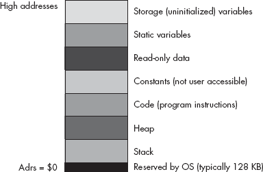
An operating system like Mac OS, Linux, or Windows puts different types of data into different areas (sections or segments) of main memory. Although it is possible to control the memory organization by running a linker and specifying various parameters, by default Windows loads a typical program into memory using the organization shown in Figure 11-6 (Linux is similar, though it rearranges some of the sections).
The operating system reserves the lowest memory addresses. Generally, your application cannot access data (or execute instructions) at the lowest addresses in memory. One reason the OS reserves this space is to help detect NULL pointer references. Programmers often initialize pointers with NULL (zero) to indicate that the pointer is not valid. Should you attempt to access memory location zero under such OSes, the OS will generate a “general protection fault” to indicate that you’ve accessed a memory location that doesn’t contain valid data.
The remaining seven areas in the memory map hold different types of data associated with your program. These sections of memory include:
The code section, which holds the program’s machine instructions.
The constant section, which holds compiler-generated read-only data.
The read-only data section, that holds user-defined data that can only be read, never written.
The static section, which holds user-defined, initialized, static variables.
The storage section, or BSS section, that holds user-defined uninitialized variables.
The stack section, where the program keeps local variables and other temporary data.
The heap section, where the program maintains dynamic variables.
Often, a compiler will combine the code, constant, and read-only data sections because all three sections contain read-only data.
Most of the time, a given application can live with the default layouts chosen for these sections by the compiler and linker/loader. In some cases, however, knowing the memory layout can allow you to develop shorter programs. For example, as the code section is usually read-only, it may be possible to combine the code, constants, and read-only data sections into a single section, thus saving any padding space that the compiler/linker may place between these sections. Although these savings are probably insignificant for large applications, they can have a big impact on the size of a small program.
The following sections discuss each of these memory areas in detail.
To understand the memory organization of a typical program, we’ve first got to define a few terms that will prove useful in our discussion. These terms are binding, lifetime, static, and dynamic.
Binding is the process of associating an attribute with an object. For example, when you assign a value to a variable, we say that the value is bound to that variable at the point of the assignment. The value remains bound to the variable until you bind some other value to it (via another assignment operation). Likewise, if you allocate memory for a variable while the program is running, we say that the variable is bound to the address at that point. The variable and address are bound until you associate a different address with the variable. Binding needn’t occur at run time. For example, values are bound to constant objects during compilation, and such bindings cannot change while the program is running.
The lifetime of an attribute extends from the point when you first bind that attribute to an object to the point when you break that bond, perhaps by binding a different attribute to the object. For example, the lifetime of a variable is from the time you first associate memory with the variable to the moment you deallocate that variable’s storage.
Static objects are those that have an attribute bound to them prior to the execution of the application. Constants are good examples of static objects; they have the same value bound to them throughout the execution of the application. Global (program-level) variables in programming languages like Pascal, C/C++, and Ada are also examples of static objects in that they have the same address bound to them throughout the program’s lifetime. The lifetime of a static object, therefore, extends from the point at which the program first begins execution to the point when the application terminates. The system binds attributes to a static object before the program begins execution (usually during compilation or during the linking phase, though it is possible to bind values even earlier).
The notion of identifier scope is also associated with static binding. The scope of an identifier is that section of the program where the identifier’s name is bound to the object. As names exist only during compilation, scope is definitely a static attribute in compiled languages. (In interpretive languages, where the interpreter maintains the identifier names during program execution, scope can be a nonstatic attribute.) The scope of a local variable is generally limited to the procedure or function in which you declare it (or to any nested procedure or function declarations in block structured languages like Pascal or Ada), and the name is not visible outside the subroutine. In fact, it is possible to reuse an identifier’s name in a different scope (that is, in a different function or procedure). In such a case as this, the second occurrence of the identifier will be bound to a different object than the first use of the identifier.
Dynamic objects are those that have some attribute assigned to them while the program is running. The program may choose to change that attribute (dynamically) while the program is running. The lifetime of that attribute begins when the application associates the attribute with the object and ends when the program breaks that association. If the program associates some attribute with an object and then never breaks that bond, the lifetime of the attribute is from the point of association to the point the program terminates. The system binds dynamic attributes to an object at run time, after the application begins execution.
Note that an object may have a combination of static and dynamic attributes. For example, a static variable will have an address bound to it for the entire execution time of the program. However, that same variable could have different values bound to it throughout the program’s lifetime. For any given attribute, however, the attribute is either static or dynamic; it cannot be both.
The code section in memory contains the machine instructions for a program. Your compiler translates each statement you write into a sequence of one or more byte values. The CPU interprets these byte values as machine instructions during program execution.
Most compilers also attach a program’s read-only data to the code section because, like the code instructions, the read-only data is already write-protected. However, it is perfectly possible under Windows, Linux, and many other operating systems to create a separate section in the executable file and mark it as read-only. As a result, some compilers do support a separate read-only data section. Such sections contain initialized data, tables, and other objects that the program should not change during program execution.
The constant section found in Figure 11-6 typically contains data that the compiler generates (as opposed to a read-only section that contains user-defined read-only data). Most compilers actually emit this data directly to the code section. Therefore, in most executable files, you’ll find a single section that combines the code, read-only data, and constant data sections.
Many languages provide the ability to initialize a global variable during the compilation phase. For example, in C/C++ you could use statements like the following to provide initial values for these static objects:
static int i = 10;
static char ch[] = ( 'a', 'b', 'c', 'd' };
In C/C++ and other languages, the compiler will place these initial values in the executable file. When you execute the application, the operating system will load the portion of the executable file that contains these static variables into memory so that the values appear at the addresses associated with them. Therefore, when the program first begins execution, these static variables will magically have these values bound to them.
Most operating systems will zero out memory prior to program execution. Therefore, if an initial value of zero is suitable and your operating system supports this feature, you don’t need to waste any disk space with the static object’s initial value. Generally, however, compilers treat uninitialized variables in a static section as though you’ve initialized them with zero, thus consuming disk space. Some operating systems provide a separate section, the BSS section, to avoid this waste of disk space.
The BSS section is where compilers typically put static objects that don’t have an explicit value associated with them. BSS stands for block started by a symbol, which is an old assembly language term describing a pseudo-opcode one would use to allocate storage for an uninitialized static array. In modern OSes like Windows and Linux, the OS allows the compiler/linker to put all uninitialized variables into a BSS section that simply contains information that tells the OS how many bytes to set aside for the section. When the operating system loads the program into memory, it reserves sufficient memory for all the objects in the BSS section and fills this memory with zeros. It is important to note that the BSS section in the executable file doesn’t actually contain any data. Because the BSS section does not require the executable file to consume space for uninitialized zeros, programs that declare large uninitialized static arrays will consume less disk space.
However, not all compilers actually use a BSS section. Many Microsoft languages and linkers, for example, simply place the uninitialized objects in the static data section and explicitly give them an initial value of zero. Although Microsoft claims that this scheme is faster, it certainly makes executable files larger if your code has large, uninitialized arrays (because each byte of the array winds up in the executable file — something that would not happen if the compiler were to place the array in a BSS section).
The stack is a data structure that expands and contracts in response to procedure invocations and the return to calling routines, among other things. At run time, the system places all automatic variables (nonstatic local variables), subroutine parameters, temporary values, and other objects in the stack section of memory in a special data structure we call the activation record (which is aptly named because the system creates an activation record when a subroutine first begins execution, and it deallocates the activation record when the subroutine returns to its caller). Therefore, the stack section in memory is very busy.
Most CPUs implement the stack using a register called the stack pointer. Some CPUs, however, don’t provide an explicit stack pointer and, instead, use a general-purpose register for this purpose. If a CPU provides an explicit stack-pointer register, we say that the CPU supports a hardware stack; if only a general-purpose register is available, then we say that the CPU uses a software-implemented stack. The 80x86 is a good example of a CPU that provides a hardware stack; the MIPS Rx000 family is a good example of a CPU family that implements the stack in software. Systems that provide hardware stacks can generally manipulate data on the stack using fewer instructions than those systems that implement the stack in software. On the other hand, RISC CPU designers who’ve chosen to use a software-stack implementation feel that the presence of a hardware stack actually slows down all instructions the CPU executes. In theory, one could make an argument that the RISC designers are right; in practice, though, the 80x86 CPU is one of the fastest CPUs around, providing ample proof that having a hardware stack doesn’t necessarily mean you’ll wind up with a slow CPU.
Although simple programs may only need static and automatic variables, sophisticated programs need the ability to allocate and deallocate storage dynamically (at run time) under program control. In the C and HLA languages, you would use the malloc and free functions for this purpose, C++ provides the new and delete operators, Pascal uses new and dispose, and other languages provide comparable routines. These memory-allocation routines have a few things in common: they let the programmer request how many bytes of storage to allocate, they return a pointer to the newly allocated storage (that is, the address of that storage), and they provide a facility for returning the storage space to the system once it is no longer needed, so the system can reuse it in a future allocation call. Dynamic memory allocation takes place in a section of memory known as the heap.
Generally, an application refers to data on the heap using pointer variables (either implicitly or explicitly; some languages, like Java, implicitly use pointers behind the programmer’s back). As such, we’ll usually refer to objects in heap memory as anonymous variables because we refer to them by their memory address (via pointers) rather than by a name.
The OS and application create the heap section in memory after the program begins execution; the heap is never a part of the executable file. Generally, the OS and language run-time libraries maintain the heap for an application. Despite the variations in memory management implementations, it’s still a good idea for you to have a basic idea of how heap allocation and deallocation operate, because an inappropriate use of the heap management facilities will have a very negative impact on the performance of your applications.
An extremely simple (and fast) memory allocation scheme would maintain a single variable that forms a pointer into the heap region of memory. Whenever a memory allocation request comes along, the system makes a copy of this heap pointer and returns it to the application; then the heap management routines add the size of the memory request to the address held in the pointer variable and verify that the memory request doesn’t try to use more memory than is available in the heap region (some memory managers return an error indication, like a NULL pointer, when the memory request is too great, and others raise an exception). The problem with this simple memory management scheme is that it wastes memory, because there is no mechanism to allow the application to free the memory that anonymous variables no longer require so that the application can reuse that memory later. One of the main purposes of a heap-management system is to perform garbage collection, that is, reclaim unused memory when an application finishes using the memory.
The only catch is that supporting garbage collection requires some overhead. The memory management code will need to be more sophisticated, will take longer to execute, and will require some additional memory to maintain the internal data structures the heap-management system uses. Let’s consider an easy implementation of a heap manager that supports garbage collection. This simple system maintains a (linked) list of free memory blocks. Each free memory block in the list will require two double-word values: one double-word value specifies the size of the free block, and the other double word contains a link to the next free block in the list (that is, a pointer), see Figure 11-7.
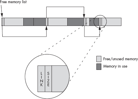
The system initializes the heap with a NULL link pointer, and the size field contains the size of the entire free space. When a memory request comes along, the heap manager first determines if there is a sufficiently large block available for the allocation request. To do this, the heap manager has to search through the list to find a free block with enough memory to satisfy the request.
One of the defining characteristics of a heap manager is how it searches through the list of free blocks to satisfy the request. Some common search algorithms are first-fit and best-fit. The first-fit search, as its name suggests, scans through the list of blocks until it finds the first block of memory large enough to satisfy the allocation request. The best-fit algorithm scans through the entire list and finds the smallest block large enough to satisfy the request. The advantage of the best-fit algorithm is that it tends to preserve larger blocks better than the first-fit algorithm, thereby allowing the system to handle larger subsequent allocation requests when they arrive. The first-fit algorithm, on the other hand, just grabs the first sufficiently large block it finds, even if there is a smaller block that would satisfy the request; as a result, the first-fit algorithm may reduce the number of large free blocks in the system that could satisfy large memory requests.
The first-fit algorithm does have a couple of advantages over the best-fit algorithm, though. The most obvious advantage is that the first-fit algorithm is usually faster. The best-fit algorithm has to scan through every block in the free block list in order to find the smallest block large enough to satisfy the allocation request (unless, of course, it finds a perfectly sized block along the way). The first-fit algorithm, on the other hand, can stop once it finds a block large enough to satisfy the request.
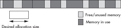
Another advantage to the first-fit algorithm is that it tends to suffer less from a degenerate condition known as external fragmentation. Fragmentation occurs after a long sequence of allocation and deallocation requests. Remember, when the heap manager satisfies a memory allocation request, it usually creates two blocks of memory — one in-use block for the request and one free block that contains the remaining bytes in the original block after the request is filled (assuming the heap manager did not find an exact fit). After operating for a while, the best-fit algorithm may wind up producing lots of smaller, leftover blocks of memory that are too small to satisfy an average memory request (because the best-fit algorithm also produces the smallest leftover blocks as a result of its behavior). As a result, the heap manager will probably never allocate these small blocks (fragments), so they are effectively unusable. Although each individual fragment may be small, as multiple fragments accumulate throughout the heap, they can wind up consuming a fair amount of memory. This can lead to a situation where the heap doesn’t have a sufficiently large block to satisfy a memory allocation request even though there is enough free memory available (spread throughout the heap). See Figure 11-8 on the next page for an example of this condition.
In addition to the first-fit and best-fit algorithms, there are other memory allocation strategies. Some execute faster, some have less (memory) overhead, some are easy to understand (and some are very complex), some produce less fragmentation, and some have the ability to combine and use noncontiguous blocks of free memory. Memory/heap management is one of the more heavily studied subjects in computer science; there is considerable literature extolling the benefits of one scheme over another. For more information on memory allocation strategies, check out a good book on OS design.
Memory allocation is only half of the story. In addition to a memory allocation routine, the heap manager has to provide a call that allows an application to return memory it no longer needs for future reuse. In C and HLA, for example, an application accomplishes this by calling the free function.
At first blush, it might seem that free would be a very simple function to write. All it looks like one has to do is append the previously allocated and now unused block onto the end of the free list. The problem with this trivial implementation of free is that it almost guarantees that the heap becomes fragmented to the point of being unusable in very short order. Consider the situation in Figure 11-9.
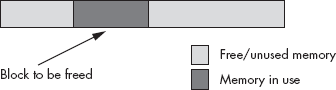
If a trivial implementation of free simply takes the block to be freed and appends it to the free list, the memory organization in Figure 11-9 produces three free blocks. However, because these three blocks are all contiguous, the heap manager should really coalesce these three blocks into a single free block; doing so allows the heap manager to satisfy a larger request. Unfortunately, from an overhead perspective, this coalescing operation requires our simple heap manager to scan through the free block list in order to determine whether there are any free blocks adjacent to the block the system is freeing. While it’s possible to come up with a data structure that reduces the effort needed to coalesce adjacent free blocks, such schemes generally involve the use of additional overhead bytes (usually eight or more) for each block on the heap. Whether or not this is a reasonable trade-off depends on the average size of a memory allocation. If the applications that use the heap manager tend to allocate small objects, the extra overhead for each memory block could wind up consuming a large percentage of the heap space. However, if the most allocations are large, then the few bytes of overhead will be of little consequence.
The performance of the algorithms and data structures the heap manager uses are only a part of the performance problem. Ultimately, the heap manager needs to request blocks of memory from the operating system. In one possible implementation, the operating system handles all memory allocation requests. Another possibility is that the heap manager is a run-time library routine that links with your application; the heap manager requests large blocks of memory from the operating system and then doles out pieces of this block as memory requests arrive from the application.
The problem with making direct memory allocation requests to the OS is that OS API calls are often very slow. If an application calls the operating system for every memory request it makes, the performance of the application will probably suffer if the application makes several memory allocation and deallocation calls. OS API calls are very slow, because they generally involve switching between kernel mode and user mode on the CPU (which is not fast). Therefore, a heap manager that the operating system implements directly will not perform well if your application makes frequent calls to the memory allocation and deallocation routines.
Because of the high overhead of an operating system call, most languages implement their own version of malloc and free (or whatever they call them) within the language’s run-time library. On the very first memory allocation, the malloc routine will request a large block of memory from the operating system, and then the application’s malloc and free routines will manage this block of memory themselves. If an allocation request comes along that the malloc function cannot fulfill in the block it originally created, then malloc will request another large block (generally much larger than the request) from the operating system, and add that block to the end of its free list. Because the calls to the application’s malloc and free routines only call the operating system on an occasional basis, this dramatically reduces the overhead associated with OS calls.
However, you should keep in mind that the procedure illustrated in the previous paragraph is very implementation and language specific; so it’s dangerous for you to assume that malloc and free are relatively efficient when writing software that requires high-performance components. The only portable way to ensure a high-performance heap manager is to develop an application-specific set of routines yourself.
Most standard heap management functions perform reasonably for a typical program. For your specific application, however, it may be possible to write a specialized set of functions that are much faster or have less memory overhead. If your application’s allocation routines are written by someone who has a good understanding of the program’s memory allocation patterns, the allocation and deallocation functions may be able to handle the application’s requests in a more efficient manner. Writing such routines is beyond the scope of this book (please see an OS textbook for more details), but you should be aware of this possibility.
A heap manager often exhibits two types of overhead: performance (speed) and memory (space). Until now, the discussion has mainly dealt with the performance characteristics of a heap manager; now it’s time to turn our attention to the memory overhead associated with the heap manager.
Each block the system allocates is going to require some amount of overhead above and beyond the storage the application requests. At the very least, each block the heap manager allocates requires a few bytes to keep track of the block’s size. Fancier (higher-performance) schemes may require additional bytes, but a typical number of overhead bytes will be between 4 and 16. The heap manager can keep this information in a separate internal table, or it can attach the block size and any other memory-management information directly to the blocks it allocates.
Saving this information in an internal table has a couple of advantages. First, it is difficult for the application to accidentally overwrite the information stored there; attaching the data to the heap memory blocks themselves doesn’t protect as well against the application wiping out this control information with buffer overruns or underruns (thus corrupting the memory manager’s data structures). Second, putting memory-management information in an internal data structure allows the memory manager to determine whether a given pointer is valid (whether it points at some block of memory that the heap manager believes it has allocated).
The advantage of attaching the control information to each block the heap manager allocates is that it is very easy to locate this information, because the memory manager typically places this information immediately before the allocated block. When the heap manager maintains this information in an internal table, it may require a search operation of some sort in order to locate the information.
Another issue that affects the overhead associated with the heap manager is the allocation granularity. Although most heap managers will allow you to allocate storage in blocks as small as one byte, most memory managers will actually allocate some minimum number of bytes greater than one. This minimum amount is the allocation granularity the memory manager supports. Generally, the engineer designing the memory-allocation functions chooses a granularity that will guarantee that any object allocated on the heap will begin at a reasonably aligned memory address for that object. As such, most heap managers allocate memory blocks on a 4-, 8-, or 16-byte boundary. For performance reasons, many heap managers begin each allocation on a typical cache-line boundary, usually 16, 32, or 64 bytes.
Whatever the granularity, if the application requests some number of bytes that is less than the heap manager’s granularity, or that is not a multiple of the granularity value, the heap manager will allocate extra bytes of storage so that the complete allocation is an even multiple of the granularity value. Therefore, there may be a few unrequested bytes tacked on to each allocation request to fill out the minimum-sized block the heap manager allocates. Of course, this amount varies by heap manager (and possibly even by version of a specific heap manager), so an application should never assume that it has more memory available than it requests; doing so would be silly, anyway, because the application could simply have requested more memory in the initial allocation call if it needed more.
The extra memory the heap manager allocates to ensure that the request is a multiple of the granularity size results in another form of fragmentation called internal fragmentation. Like external fragmentation, internal fragmentation results in the loss of small amounts of memory throughout the system that cannot satisfy future allocation requests. Assuming random sized memory allocations, the average amount of internal fragmentation that will occur on each allocation is half the granularity size. Fortunately, the granularity size is quite small for most memory managers (typically 16 bytes or fewer), so after thousands and thousands of memory allocations you’ll only lose a couple dozen or so kilobytes to internal fragmentation.
Between the costs associated with allocation granularity and the memory control information, a typical memory request may require between 4 and 16 bytes, plus whatever the application requests. If you are making large memory allocation requests (hundreds or thousands of bytes), the overhead bytes won’t consume a large percentage of memory on the heap. However, if you allocate lots of small objects, the memory consumed by internal fragmentation and control information may represent a significant portion of your heap area. For example, consider a simple memory manager that always allocates blocks of data on 4-byte boundaries and requires a single 4-byte length value that it attaches to each allocation request for control purposes. This means that the minimum amount of storage the heap manager will require for each allocation is eight bytes. If you make a series of malloc calls to allocate a single byte, the application will not be able to use almost 88 percent of the memory it allocates. Even if you allocate 4-byte values on each allocation request, the heap manager consumes 67 percent of the memory for overhead purposes. However, if your average allocation is a block of 256 bytes, the overhead only requires about 2 percent of the total memory allocation. Moral of the story: The larger your allocation request, the less impact the control information and internal fragmentation will have on your heap.
Computer science journals contain lots of examples of software engineering studies where the authors determined that memory allocation and deallocation requests caused a significant loss of performance in their systems. In such studies, the authors often obtained performance improvements of 100 percent or better by simply implementing their own simplified, application-specific, memory-management algorithms rather than calling the standard run-time library or OS kernel memory allocation code. Let’s hope this section has made you aware of this potential problem in your own code.
Like the previous couple of chapters, this chapter deals with computer architecture issues. Almost any decent college textbook on computer architecture will go into considerable depth discussing caches and the memory hierarchy. Patterson and Hennessy’s Computer Architecture: A Quantitative Approach is one of the better-regarded texts on this subject. For information about virtual memory management, a good operating systems textbook will be useful as well. For information about the specific paging mechanism and support for virtual memory that your particular CPU provides, see the CPU manufacturer’s data books for the CPU.
[43] Actually, some systems now offer an external level-three cache. External level-three caches are present on some systems where the L1 and L2 caches are part of the CPU package and the system implementor wants to add more cache to the system.
[44] Note, however, that in some degenerate cases virtual memory can be much slower than file access.
[45] Strictly speaking, you actually get a 36-bit address space on Pentium Pro and later processors, but Windows and Linux limit you to 32 bits, so we’ll use that limitation here.