21	Nanodevices Describing Function and Liénard Equation Alberto Delgado

CONTENTS

21.1 Introduction

21.2 Describing Function

21.2.1 Memristor

21.2.2 Nanodevices Based on DNA or CNTs

21.3 The Liénard Equation

21.3.1 Conditions for a Limit Cycle

21.3.2 Quadratic Memristor

21.3.3 Nonlinear Nanodevice

21.4 Simulations

21.4.1 Limit Cycle

21.4.2 Stable Fixed Point

21.5 Conclusions

References

21.1  INTRODUCTION

Nanotechnology is a promising research area with applications in different disciplines. In electrical and electronic engineering, nanodevices are new building blocks for circuits that increase the designer possibilities beyond traditional elements. In this chapter, two methods to study the behavior of nonlinear circuits and systems are illustrated for memristors, and nanodevices based on deoxyribonucleic acid (DNA) or carbon nanotubes (CNTs).

The two points of view are: (i) frequency analysis with the describing function (DF) [1,2], and (ii) time analysis with the Liénard equation [3]. The purpose of these tools is to predict the behavior of circuits and systems with nonlinear nanodevices or even to guide the design of nanodevices to synthesize any desired dynamics. Also, the tunable nanodevices could increase the complexity and applications of new circuits.

In the literature, it is common to find experimental v−i characteristics for nanodevices; these plots show nonlinear behavior that can be described by piecewise linear equations. Some typical nanodevices are based on oxide films [4, 5 and 6], DNA [7], or CNTs [8]. In other nanodevices, the nonlinear v−i relationship can be expressed as formulas, v = φ(i), ϕ = f(q); the current is related to the charge, i = dq/dt, and the voltage is related to the flux, v = dϕ/dt.

This chapter is divided as follows. Section 21.2 presents the definition of DF and its calculation, step by step, for a general nonlinearity. Then, the general formula is applied to memristors, and DNA or CNTs-based nanodevices. Section 21.3 introduces the Liénard equation for series RLC circuits with nanodevices; two types of nonlinearities are considered v = φ(i) and ϕ = f(q); also, five conditions for the existence of limit cycles are formulated. Section 21.4 presents the simulations to support the theoretical predictions for self-sustained oscillations. Finally, Section 21.5 includes some conclusions and future work.

21.2  DESCRIBING FUNCTION

In nonlinear control theory, the DF is used to predict the behavior of a nonlinear device in closed loop with a linear system, see Figure 21.1. The characteristic polynomial (denominator) of the closed-loop transfer function produces two equations; the solution yields the frequency and amplitude (ω,a) of the limit cycle or self-sustained oscillation [1]. This approach is called analysis in the frequency domain; the input voltage is periodic with known amplitude.

The closed-loop transfer function obeys the expression,

$\frac{Y(\text{j}\omega )}{R(\text{j}\omega )}=\frac{\Psi (a)G(\text{j}\omega )}{1+\Psi (a)(\text{j}\omega )}$

(21.1)

where Ψ(a) is the DF of the nonlinear nanodevice and G(jω) is the linear system transfer function in the frequency domain. The closed loop has a limit cycle when,

$1+\Psi (a)G(\text{j}\omega )=0$

(21.2)

The function G(jω) is a complex quantity with real and imaginary parts; if the DF is real, there are two equations,

$\begin{array}{l}\Psi (a)\cdot \mathrm{Re}[G(\text{j}\omega )]=-1\hfill \\ \mathrm{Re}[G(\text{j}\omega )]=\frac{-1}{\Psi (a)}\hfill \end{array}$

(21.3)

$\begin{array}{l}\Psi (a)\cdot \mathrm{Im}[G(\text{j}\omega )]=0\hfill \\ \mathrm{Im}[G(\text{j}\omega )]=0\hfill \end{array}$

(21.4)

Solving Equation 21.4 produces the limit cycle frequency and Equation 21.3 yields the oscillation amplitude [2]. When a closed-loop system like Figure 21.1 is given, in a practical situation, the first step is to find the DF Ψ(a) for the nonlinearity.

The definition of a real DF Ψ(a) for odd, time invariant, memoryless nonlinearities is the following [1]:

$\Psi (a)=\frac{2}{\pi a}{\displaystyle {\int }_0^{\pi }i(\theta )\sin \theta \text{d}\theta }$

(21.5)

This analysis is valid for the input voltage,

$v(\theta )=a\sin \theta$

(21.6)

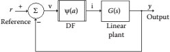
FIGURE 21.1  Linear plant in closed loop with a nanodevice, s is the Laplace operator.

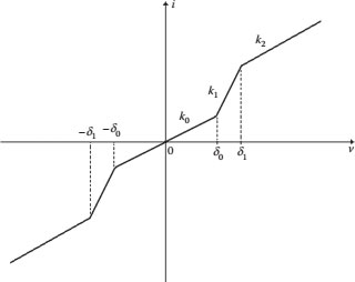
FIGURE 21.2  Nonlinear static v−i characteristic for a general nanodevice.

Figure 21.2 shows a voltage–current characteristic for a general nanodevice where (k₀,k₁,k₂) are slopes; this v−i function can be studied using the DF as follows.

To evaluate integral (21.5), it is necessary to find the current i(θ) for different intervals following the input voltage (21.6),

$\begin{array}{l}\begin{array}{cc}0\le \theta <{\beta }_0;& i=k_0\cdot v\end{array}\hfill \\ \begin{array}{cc}{\beta }_0\le \theta <{\beta }_1;& i={\delta }_0(k_0-k_1)+k_1\cdot v\end{array}\hfill \\ \begin{array}{cc}{\beta }_1\le \theta <\pi -{\beta }_1;& i={\delta }_0{k}_0+({\delta }_1-{\delta }_0)k_1+k_2\cdot (v-{\delta }_1)\end{array}\hfill \\ \begin{array}{cc}\pi -{\beta }_1\le \theta <\pi -{\beta }_0;& i={\delta }_0(k_0-k_1)+k_1\cdot v\end{array}\hfill \\ \begin{array}{cc}\pi -{\beta }_0\le \theta \le \pi ;& i=k_0\cdot v\end{array}\hfill \end{array}$

(21.7a)

where

$\begin{array}{cc}{\beta }_0={\sin }^{-1}\left(\frac{{\delta }_0}{a}\right);& {\beta }_1={\sin }^{-1}\left(\frac{{\delta }_1}{a}\right);\end{array}$

(21.7b)

Writing again Equation 21.5 and using Equation 21.7 yields,

$\begin{array}{lll}\Psi (a)\hfill & =\hfill & \frac{2}{\pi a}{\displaystyle {\int }_0^{{\beta }_0}{k}_{0}a{\sin }^2\theta \text{d}\theta }\hfill \\ \hfill & \hfill & +\frac{2}{\pi a}{\displaystyle {\int }_{\pi -{\beta }_0}^{\pi }{k}_{0}a{\sin }^2\theta \text{d}\theta }\hfill \\ \hfill & \hfill & +\frac{2}{\pi a}{\displaystyle {\int }_{{\beta }_0}^{{\beta }_1}[{\delta }_0(k_0-k_1)+k_{1}a\sin \theta ]\sin \theta \text{d}\theta }\hfill \\ \hfill & \hfill & +\frac{2}{\pi a}{\displaystyle {\int }_{\pi -{\beta }_0}^{\pi -{\beta }_1}[{\delta }_0(k_0-k_1)+k_{1}a\sin \theta ]\sin \theta \text{d}\theta }\hfill \\ \hfill & \hfill & +\frac{2}{\pi a}{\displaystyle {\int }_{{\beta }_1}^{\pi -{\beta }_1}[{\delta }_0{k}_0+({\delta }_1-{\delta }_0)k_1+k_{2}a\sin \theta -{\delta }_1{k}_2]\sin \theta \text{d}\theta }\hfill \end{array}$

(21.8)

Integrating each term [9], and after some algebra, the DF for the nonlinearity of Figure 21.2 obeys,

$\begin{array}{lll}\Psi (a)\hfill & =\hfill & \frac{2k_0}{\pi }\left[{\sin }^{-1}\left(\frac{{\delta }_0}{a}\right)-\frac{{\delta }_0}{a}\sqrt{1-{\left(\frac{{\delta }_0}{a}\right)}^2}\right]\hfill \\ \hfill & \hfill & +\frac{4}{\pi a}\left[{\delta }_0{k}_0+({\delta }_1-{\delta }_0)k_1-\frac{{\delta }_1{k}_2}{2}\right]\sqrt{1-{\left(\frac{{\delta }_1}{a}\right)}^2}\hfill \\ \hfill & \hfill & -\frac{2k_2}{\pi }{\sin }^{-1}\left(\frac{{\delta }_1}{a}\right)+k_2;\left|a\right|>{\delta }_1\hfill \end{array}$

(21.9)

Formula (21.9) can be used to find the DF of known nanodevices by replacing the value δ₀, δ₁, k₀, k₁, k₂ from the corresponding v−i characteristics.

21.2.1  MEMRISTOR

Figure 21.3 shows the v−i response for a memristor [4, 5 and 6].

To reduce Figure 21.2 to Figure 21.3,

$\begin{array}{cc}{k}_1=k_2,& {\delta }_0={\delta }_1\end{array}$

Replacing these relationships in Equation 21.9,

$\begin{array}{cc}\Psi (a)=\frac{2(k_0-k_1)}{\pi }\left[{\sin }^{-1}\left(\frac{{\delta }_0}{a}\right)+\frac{{\delta }_0}{a}\sqrt{1-{\left(\frac{{\delta }_0}{a}\right)}^2}\right]+k_1;& \left|a\right|>{\delta }_0\end{array}$

(21.10)

Equation 21.10 is the memristor DF when the frequency of the input voltage is constant.

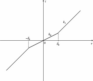
FIGURE 21.3  Nonlinear v−i characteristic for a memristor with fixed frequency.

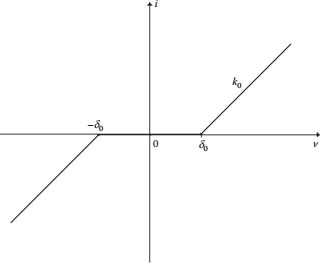
FIGURE 21.4  Nonlinear v–i characteristic of DNA or CNT-based nanodevice.

21.2.2  NANODEVICES BASED ON DNA OR CNTS

Other types of nanodevices use the molecule of life (DNA) or CNTs between a pair of electrodes [7,8]. For these electronic devices, the general DF (21.9) can be applied to the v−i characteristic, see Figure 21.4.

To reduce Figure 21.2 to Figure 21.4,

$\begin{array}{ccc}{k}_0=0;& k_1=k_2=k_0;& {\delta }_0={\delta }_1\end{array}$

Replacing these parameters in Equation 21.9,

$\begin{array}{cc}\Psi (a)=k_0-\frac{2k_0}{\pi }\left[{\sin }^{-1}\left(\frac{{\delta }_0}{a}\right)-\frac{{\delta }_0}{a}\sqrt{1-{\left(\frac{{\delta }_0}{a}\right)}^2}\right];& \left|a\right|>{\delta }_0\end{array}$

(21.11)

Equation 21.11 is the DF for the typical nonlinearity of DNA or CNT-based nanodevices.

21.3  THE LIÉNARD EQUATION

The second approach to study circuits and systems with nonlinear nanodevices is known as time domain analysis and involves nonlinear differential equations; here, numerical solutions are required when the differential equation is not standard.

The forced Liénard equation [3] has the structure,

$\frac{{\text{d}}^{2}x}{\text{d}{t}^2}+a_1(x)\frac{\text{d}x}{\text{d}t}+a_0(x)=u$

(21.12)

where a₁(x); a₀(x) are nonlinear functions; u is the forcing input.

21.3.1  CONDITIONS FOR A LIMIT CYCLE

The solution of Equation 21.12 presents a limit cycle or self-sustained oscillation if the following five conditions are satisfied,

1.  The coefficients a₁(x); a₀(x) are continuously differentiable for all x.

2.  Coefficient a₀(x) has odd symmetry,

$a_0(x)=-a_0(-x)\forall x$

(21.13)

3.  Coefficient a₀(x) is positive for x positive,

$a_0(x)>0\forall x>0$

(21.14)

4.  Coefficient a₁(x) has even symmetry,

$a_1(x)=a_1(-x)\forall x$

(21.15)

5.  The function F(x) has one positive zero at x = a,

$F(x)={\displaystyle {\int }_0^x{a}_1(\lambda )\text{d}\lambda }$

(21.16)

F(x) < 0, for 0 < x < a;

F(x) > 0 and nondecreasing for x > a;

F(x) → ∞ as x → ∞;

The Liénard equation 21.12 appears naturally in series RLC circuits with memristors or nanodevices with nonlinear v–i characteristics.

21.3.2  QUADRATIC MEMRISTOR

Consider the circuit shown in Figure 21.5 with a memristor ϕ = f(q).

The corresponding differential equation,

$R.i+L\frac{\text{d}i}{\text{d}t}+\frac{1}{C}{\displaystyle {\int }_0^t\text{i}(\tau )\text{d}\tau }+\frac{\text{d}f(q)}{\text{d}q}i=u$

(21.17)

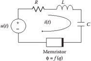
FIGURE 21.5  RLC circuit with a memristor ϕ = f(q).

Here, the memristance M = df(q)/dq is quadratic in relation with the charge,

$M(q)=\frac{\partial f(q)}{\partial q}=k(q^2-\alpha )$

(21.18)

where (k,α) are constants; replacing Equation 21.18 by Equation 21.17 with i = dq/dt yields,

$\frac{{\text{d}}^{2}q}{\text{d}t}+\left(\frac{R+k(q^2-\alpha )}{L}\right)\frac{\text{d}q}{\text{d}t}+\frac{1}{LC}q=u$

(21.19)

This Liénard equation, for the memristive circuit shown in Figure 21.5, has coefficients a₀(x) and a₁(x) that satisfy the limit cycle conditions 1–4. Equation 21.19 can be written as Equation 21.12 with coefficients (21.20).

$\begin{array}{l}{a}_0(x)=\frac{1}{LC}x\hfill \\ a_1(x)=\left(\frac{R+k(x^2-\alpha )}{L}\right)\hfill \end{array}$

(21.20)

Condition five for a limit cycle (21.16) requires the integration of a₁(x),

$F(x)={\displaystyle {\int }_0^x\frac{1}{L}[R+k({\lambda }^2-\alpha )]\text{d}\lambda }=\frac{1}{L}\left[(R-k\alpha )x+\frac{k}{3}{x}^3\right]$

(21.21)

Finding the positive zero,

$\begin{array}{l}\frac{1}{L}\left[(R-k\alpha )x+\frac{k}{3}{x}^3\right]=0\hfill \\ x=\sqrt{\frac{3(k\alpha -R)}{k}}\hfill \end{array}$

(21.22)

Formula (21.22) is dependent on the memristor parameters (k,α) and the resistive part R of the circuit, that is, the elements that damp oscillations or dissipative elements.

21.3.3  NONLINEAR NANODEVICE

Figure 21.6 is a series RLC circuit with a general nonlinear nanodevice v = φ(i).

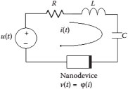
FIGURE 21.6  RLC circuit with a nonlinear nanodevice v = φ(i).

The differential equation in this case includes the function φ(i),

$R.i+L\frac{\text{d}i}{\text{d}t}+\frac{1}{C}{\displaystyle {\int }_0^t\text{i}(\tau )\text{d}\tau }+\text{φ}(i)=u$

(21.23)

If the input u is constant, then the derivative with respect to time of Equation 21.23 follows the expression,

$\begin{array}{l}\frac{{\text{d}}^{2}i}{\text{d}{t}^2}+\frac{1}{L}[R+\text{Γ}(i)]\frac{\text{d}i}{\text{d}t}+\frac{1}{LC}i=0\hfill \\ \text{Γ}(i)=\frac{\partial \text{φ}(i)}{\partial i}\hfill \end{array}$

(21.24)

In some cases, from the nanodevice experimental v–i characteristic, it could be possible to interpolate a continuous function v = φ(i).

21.4  SIMULATIONS

In this section, two series RLC circuits with quadratic memristors are simulated [10] to verify the presence of limit cycles if the five conditions of the Liénard equation are satisfied [3]. The parameters for the simulation are: R = 4 Ω, L = 2 H, and C = 0.5 F.

21.4.1  LIMIT CYCLE

In the first case, the constants for M(q) are (k, α) = (10, 0.5); the positive zero is located at x = 0.55. Integral (21.16) is the cubic equation (21.25) shown in Figure 21.7; notice that F(x) satisfies condition five for a limit cycle.

$F(x)=-0.5x+\frac{5}{3}{x}^3$

(21.25)

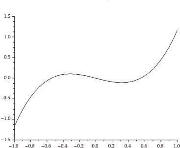
FIGURE 21.7  F (x) for Liénard equation with a limit cycle.

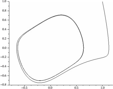
FIGURE 21.8  Limit cycle from an initial condition (1,1).

Writing the unforced Liénard equation for this memristive circuit (k,α) = (10, 0.5) with initial conditions (21.26),

$\begin{array}{l}\frac{{\text{d}}^{2}x}{\text{d}t}+(-0.5+5x^2)\frac{\text{d}x}{\text{d}t}+x=0\hfill \\ \begin{array}{cc}\frac{\text{d}x(0)}{\text{d}t}=1;& x(0)=1\end{array}\hfill \end{array}$

(21.26)

Figure 21.8 is the solution of Equation 21.26; there is a limit cycle because a₁(x); a₀(x) satisfy all the required conditions.

21.4.2  STABLE FIXED POINT

In the second case, the constants for M(q) are (k,α) = (2, 0.5); there is no positive zero; instead, x = ± j 2.12. Integral (21.16) is the cubic equation (21.27) shown in Figure 21.9; notice that F(x) does not satisfy condition five for a limit cycle.

$F(x)=1.5x+\frac{1}{3}{x}^3$

(21.27)

Writing the unforced Liénard equation for this memristive circuit (k,α) = (2, 0.5) with initial conditions (21.28),

$\begin{array}{l}\frac{{\text{d}}^{2}x}{\text{d}{t}^2}+(1.5+5x^2)\frac{\text{d}x}{\text{d}t}+x=0\hfill \\ \begin{array}{cc}\frac{\text{d}x(0)}{\text{d}t}=1;& x(0)=1\end{array}\hfill \end{array}$

(21.28)

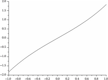
FIGURE 21.9  F(x) does not satisfy the conditions for a limit cycle.

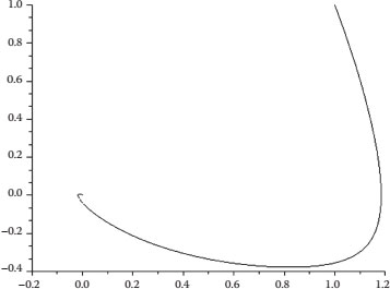
FIGURE 21.10  Stable fixed point for an initial condition (1,1).

Figure 21.10 is the solution of Equation 21.28; there is no limit cycle because a₁(x); a₀(x) do not satisfy the required conditions.

21.5  CONCLUSIONS

This chapter has presented two methods, frequency-domain analysis and time-domain analysis, to study circuits and systems with nonlinear nanodevices; the corresponding mathematical concepts are the DF and the Liénard equation, respectively.

The DF for a general v–i characteristic was calculated and the final formula, with particular parameters, was used to derive the DFs for a memristor and for DNA and CNTs-based nanodevices.

In the time domain, the Liénard equation was formulated for RLC series circuits with nanodevices; two types of nonlinearities were considered, v = φ(i) and ϕ = f(q). Conditions for the existence of a limit cycle were formulated and the theory was illustrated with simulations.

Future work could consider a time-varying DF to improve the modeling of frequency-dependent nanodevices such as the memristor [5]; also, the design of nanodevices to synthesize particular v–i characteristics is an open problem.

REFERENCES

1.  Khalil, H.K. Nonlinear Systems. Macmillan Publishing, New York, NY, 1992.

2.  Delgado, A. The memristor as controller. IEEE Nanotechnology Materials and Devices Conference, Monterey, California, Oct. 12–15, 2010.

3.  Strogatz, S.H. Nonlinear Dynamics and Chaos. Perseus Books Publishing, Cambridge, 1994.

4.  Chua, L.O. Memristor—The missing circuit element. IEEE Transactions on Circuit Theory, 18(5), 507–519, 1971.

5.  Strukov, D.B., Snider, G.S., Stewart, D.R., and Williams, R.S. The missing memristor found. Nature, 453, 80–83, 2008.

6.  Jeong, H. J., Lee, J. Y., Ryu, M. K., and Choi, S. Y. Bipolar resistive switching in amorphous titanium oxide thin film. Physica Status Solidi RRL 4(1–2), 28–30, 2010.

7.  Cohen, H., Nogues, C., Naaman, R., and Porath, D. Direct measurement of electrical transport through single DNA molecules of complex sequence. Proceedings of the National Academy of S ciences, USA, 102(33), 11589–11593, 2005.

8.  Kaun, C.-C., Larade, B., Mehrez, H., Taylor, J., and Guo, H. Current—voltage characteristics of carbon nanotubes with substitutional nitrogen. Physical Review B, 65, 205416 (1–5), 2002.

9.  Wolfram Alpha LLC. 2012. Wolfram|Alpha. http://www.wolframalpha.com/input/?i=integrate (access May 22, 2012). The use of Wolfram|Alpha does not imply in any way that Wolfram endorses the particular substance or general quality of this work.

10.  Consortium Scilab–Digiteo 2011. Scilab: Free and Open Source software for numerical computation (OS, Version 5.XX) [Software]. Available from: http://www.scilab.org.