CONTENTS

39.1  Introduction

39.2  Model and Methodology

39.3  Simulation Results

39.3.1    Electron Resonances

39.3.2    Kinetic Inductance

Acknowledgments

References

39.1  INTRODUCTION

Recently, a terahertz response of single-walled carbon nanotubes has been successfully observed and measured [1,2]. Carbon nanotubes (CNTs) have emerged as one of the most active areas of nanoscale science and technology research [3,4]. They are truly nanoscale materials with typical diameters of 1–2 nm, and can be regarded as being close to ideal 1-D conductors with an unprecedented mean free path of about 1 μm at 300 K. Their cross-sectional dimensions are about an order of magnitude smaller than the limiting dimensions at which complementary metal oxide semiconductor (CMOS) technology is likely to encounter insuperable scaling limits in a few years. Not surprisingly, it has turned out to be quite difficult to realize actual working applications by using materials at such a radically different scale; this is still a largely unmet challenge! For example, CNT field-effect transistors (CNT-FETs) have been predicted to perform up to terahertz frequencies [5,6], but experiments show switching speeds [4] (digital circuits) or cutoff frequencies (analog circuits) that are at least a couple of orders of magnitude below that predicted intrinsic performance. Measurements on CNTs have been extended to about 60 GHz, and much higher frequencies (up to several THz) are required to verify the properties of CNTs as predicted by existing theories. These theories predict plasmon waves propagating along the tubes at slow speeds of roughly 0.01c (c is the speed of light), a unique feature of 1-D conductors [7]. The transmission line model for a metallic single-walled CNT (m-SWCNT) introduced in Ref. [7] includes a unique kinetic inductance element that is about 1000 times greater than the magnetic inductance usually considered for macroscopic conductors. It also incorporates a quantum capacitance. Based on this model, one predicts that plasmon resonances should occur at terahertz frequencies for CNTs as short as 1 μm. It is a current, so far unmet, challenge for experimentalists to measure and take advantage of these resonances. The unusual antenna properties of CNTs have been predicted in Ref. [8]. Surface wave types of fields near the tubes are predicted to be enhanced by hundreds of times [9], and this has also not yet been demonstrated experimentally. Such surface waves are promising for many applications, similar to those that are presently under intense development in the optical/NIR range, employing surface plasmon polaritons (SPPs) [10]. The utilization of the plasmon phenomena shows potential for shrinking circuit sizes to a small fraction of a wavelength, at THz as well as in the visible/NIR. Many unique applications of CNTs in the terahertz frequency range thus appear possible when these types of plasmon phenomena are well understood.

In this chapter, we present large-scale quantum atomistic time-domain simulations to gain an in-depth picture of electron transport phenomena at very high frequencies in CNTs. These numerical models are expected to provide fundamental insights for understanding plasmonic and other many-body excitations and then enhance the reliability in designing tunable carbon-based electronic devices. The simulations are performed with short time steps to be able to correctly represent phenomena up to over 100 THz. We especially emphasize an investigation of any resonances, as well as the kinetic inductance.

For large systems under time-dependent external perturbations such as electromagnetic (EM) fields, pulsed lasers, AC signals, particle scattering, and so on, a full quantum treatment of the problem is still considered to be very challenging. Reliable modeling approaches in the time domain are often limited in terms of trade-off between robustness and performances [11,12]. In our work, effective modeling and propagation schemes are carried out to simulate the CNT THz response. Our propagation schemes consist of performing a direct integration of the time-ordered evolution operator. The numerical treatment of time-ordered evolution operators often gives rise to the matrix exponential. The most obvious way to address this numerical problem would be to directly diagonalize the Hamiltonian while selecting the relevant number of modes needed to accurately expand the solutions. Direct diagonalization techniques, however, have been known to be very computationally demanding, especially for large systems. Consequently, the mainstream in time-dependent simulations uses traditional approximations such as split operator techniques or a perturbation theory. Here, we rather perform exact diagonalizations by taking advantage of our new linear scaling eigenvalue solver FEAST [13]. By using FEAST, the solution of the eigenvalue problem is reformulated into solving a set of well-defined, independent linear systems along a complex energy contour. Additionally, obtaining the spectral decomposition of the matrix exponential becomes a suitable alternative to PDE-based techniques, such as the Crank–Nicolson schemes [14], and can also potentially be performed using a time-domain parallelism.

39.2  MODEL AND METHODOLOGY

In time-dependent quantum systems, the electrons obey the time-dependent Schrödinger equation:

Besides appropriate boundary conditions, the time-dependent Schrödinger equation requires an initial value condition Ψ(t = 0) = Ψ₀ that completely determines the dynamics of the system.

Using a single electron picture, and in the time-dependent density functional theory (TDDFT) framework [15], the solutions of the stationary Kohn–Sham Schrödinger-type Equation 39.2 are taken as initial wave functions ${\text{Ψ}}_0=\{{\psi }_1^{(0)},{\psi }_2^{(0)},\dots ,{\psi }_{N_e}^{(0)}\}$ and will be propagated over time.

For a system of interest that is composed of N_e electrons, the electron dynamics can be described by a set of one-body equations, the Kohn–Sham equations. It has the same form as the Schrödinger equation, where $\text{Ψ}=\{{\psi }_1,{\psi }_2,\dots ,{\psi }_{N_e}\}$ and with ψ_j the solution of

The Kohn–Sham potential v_KS is a functional of the time-dependent density and it is conventionally separated in the following way:

where the first term represents the external potential, the second term is the Hartree potential that accounts for the electrostatic interaction between the electrons, and the last term is defined as the exchange-correlation potential that accounts for all the nontrivial many-body effects. The density of the interacting system can be obtained from the time-dependent Kohn–Sham wave functions

TDDFT can indeed be viewed as a reformulation of time-dependent quantum mechanics where the basic variable is no longer the many-body wave function, but the time-dependent electron density n(r,t). For any fixed, initial many-body state, the Runge–Gross theorem [15] shows that there is one-to-one correspondence between densities and the potential, which means that the external potential uniquely determines the density. The Kohn–Sham approach chooses a noninteracting system, which has a density that is equal to the interacting system.

Formally, the solution of Equation 39.1 can be written as

where the evolution operator ${\displaystyle \widehat{U}}$ is unitary and can be represented using a time-ordered exponential $\mathcal{T}\exp$, which is a nontrivial mathematical object. In most cases, the problem is addressed using very small time steps and the time-independent Hamiltonian approximation within the intervals. Intermediate physical solutions are computed in addition to the final solution Ψ(t) to describe the evolution of the system over [0,t]. This can be accomplished by dividing [0,t] into smaller time intervals since using the intrinsic properties of the evolution operator, one can apply the following decomposition:

If the Δ_t chosen is very small, it is reasonable to consider the ${\displaystyle \widehat{H}}(\tau )$ constant within the time interval [t,t +Δ_t], leading to

Equation 39.8 requires the solution of eigenvalue problems, while the exact Hamiltonian diagonalization is often considered to be computationally challenging. For large systems, approximations such as the Crank–Nicolson or split operator are commonly made since the direct factorization of the evolution operator is not practical using conventional eigenvalue solvers. In our previous work [16], we have proposed new effective and direct numerical propagation schemes that go beyond the perturbation theory and linear response. We also perform the exact diagonalizations of Hamiltonians by taking advantage of a new linear scaling eigenvalue solver, FEAST.

Denoting H the N × N Hamiltonian matrix obtained after the discretization of at a given time t and where N could represent the number of basis functions (or number of nodes using real-space mesh techniques), H can then be diagonalized as follows:

where the columns of the matrix P = {p₁,p₂,…,p_M} represent the eigenvectors of H associated with the M lowest eigenvalues regrouped within the diagonal matrix D = {d₁,d₂,…,d_M}. Now, we can get the resulting matrix form of the time propagation equation, which is given by

Using the property (39.7), the solution Ψ(t) can finally be obtained as a function of Ψ₀:

where $D_i=P_i^{T}H(t_i)P_i.S$ is a symmetric positive-definite matrix that satisfies P^TSP = I.

In addition to the (basic) direct propagation scheme above, two highly efficient propagation schemes using larger time intervals have also been proposed in Ref. [16].

39.3  SIMULATION RESULTS

Based on the modeling strategies presented here, we have recently developed a highly efficient numerical framework for performing first-principle TDDFT using all-electron calculations and 3-D finite element discretization. While this framework is already capable of reproducing optical absorption spectra of molecules (from H2 to C60) [17], it is still currently being optimized to effectively address THz responses for much larger-scale systems running on high-end parallel architectures.

In this section, however, we present the preliminary results obtained using our 3-D time-dependent, numerical framework, making use of an atomistic, empirical pseudopotential, which has allowed use to capture the THz response of metallic CNT and accurately reproduce experimental results on the Fermi velocity and kinetic inductance. In our model, we use an empirical pseudopotential [18], and propose to compute the response of a time-dependent, external perturbation applied to the system (EM radiation). The evolution of all t = 0 wave functions (i.e., all electrons present in the system) are considered with the time-dependent Hamiltonian. Our model also uses real-space mesh techniques for discretization (finite element method), and a time-dependent version of the atomistic mode approach described in Ref. [19]. Moreover, if the empirical pseudopotential U_eps is supposed to be time independent, the total atomistic potential can then be decomposed as follows:

where x is the longitudinal direction of the tube, L represents the distance between contacts (x ∈ [0,L]), and ω = 2πf, with f being the corresponding frequency of the AC signal and U₀ its amplitude. The time-dependent external potential applied to the CNT then maintains zero in the middle of the tube but oscillates at both ends alternatively to the ±U₀ values.

39.3.1  ELECTRON RESONANCES

We apply the direct propagation scheme to an isolated (5,5) metallic carbon nanotube (see Figure 39.1). In the noninteracting Kohn–Sham system, the N ground-state Kohn–Sham orbitals are taken as the initial states and are propagated over time. A very short pulse (time domain) is injected into the device. We calculate the current density in the middle of the tube, and then Fourier transform the current density to get the responses of the CNT.

We studied CNTs with different lengths, which are described in Table 39.1 (the CNT length in the table represents the entire computational domain).

Since we have the wavefunction at any time, we could get density and current at any time t. The probability current density ${\displaystyle \overrightarrow{j}}$ of the wave function Ψ is defined as

After integrating over the cross section, we have the current in the middle of the tube versus time. Figure 39.2 shows the current versus time at the middle of the tube for 12 unit cell and 24 unit cell SWCNTs, where the width of the pulse is 0.04 fs, and the total propagation time is 1.25 × 10⁻¹³ s.

Then, we Fourier transform the current:

$\begin{array}{cc}{X}_k={\displaystyle {\displaystyle \sum _{n=0}^{N-1}}{I}_n{e}^{-\frac{2\pi i}{N}kn}}& k=0\end{array},\dots ,N-1$

with the results shown in Figure 39.3.

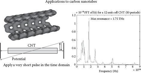
FIGURE 39.1  Schematic representation of the simulation setup. (Chen, Z. et al., Real-time quantum simulation of terahertz response in single wall carbon nanotube, 2011 11th IEEE Conference on Nanotechnology (IEEE-NANO), Portland, OR, pp. 1339–1342. © (2011) IEEE. With permission.)

TABLE 39.1
(5,5) CNTs of Different Lengths

Source:  Chen, Z. et al., Real-time quantum simulation of terahertz response in single wall carbon nanotube, 2011 11th IEEE Conference on Nanotechnology (IEEE-NANO), Portland, OR, pp. 1339–1342. © (2011) IEEE. With permission.

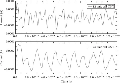
FIGURE 39.2  Current density in the middle of nanotube versus time. (Chen, Z. et al., Real-time quantum simulation of terahertz response in single wall carbon nanotube, 2011 11th IEEE Conference on Nanotechnology (IEEE-NANO), Portland, OR, pp. 1339–1342. © (2011) IEEE. With permission.)

The frequencies of the maximum response of 12 unit cell and 24 unit cell SWCNTs are 175 and 88 THz, respectively, which correspond to the resonance frequency. We know that the lowest frequency for a Fabry–Perot resonance can be obtained from

so the phase velocity for the 12 unit cell CNT is

$v=f*\lambda =f*2L=1.13\times {10}^8\text{cm/s}.$

And, similarly, the phase velocity for the 24 unit cell CNT is

$v=1.14\times {10}^8\text{cm/s}.$

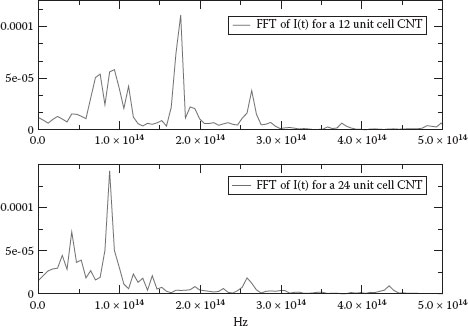
FIGURE 39.3  Fourier transform of the current density. (Chen, Z. et al., Real-time quantum simulation of terahertz response in single wall carbon nanotube, 2011 11th IEEE Conference on Nanotechnology (IEEE-NANO), Portland, OR, pp. 1339–1342. © (2011) IEEE. With permission.)

We can see that the phase velocity is constant, showing that the high-frequency electron response is dominated by single-particle excitations rather than collective plasmon modes. Burke [7] and Hanson et al. [8] have found the plasmon velocity of SWCNT to be approximately 3 × 10⁸ and 6 × 10⁸ cm/s. Our simulations show that we have obtained a phase velocity that is consistent with the Fermi velocity 8 × 10⁷ cm/s, which was also measured in a recent experiment [2]. We have also performed simulations in which the applied potential was varied sinusoidally at the resonant frequencies given above. In this case, we find responses from our simulations such as the peaks shown in Figure 39.3 below the resonances. These responses are consistent with the electron excitations due to the HOMO-LUMO gap in the system. For the 12 unit cell case, if one assumes the lower response at 100 THz, the corresponding energy is 0.414 eV, and in our simulation, we find that the HOMO-LUMO gap for this system is 0.416 eV.

39.3.2  KINETIC INDUCTANCE

From the solutions for the wave functions, one can now investigate many properties of the CNT. In particular, within the real-space mesh framework, the electron density is given by

Kinetic inductance is an important property of the CNT. The total kinetic energy can be expressed in terms of the current I and equivalence to the inductance used:

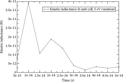
FIGURE 39.4  Simulation result of the kinetic inductance versus time. (Chen, Z. et al., Real-time quantum simulation of terahertz response in single wall carbon nanotube, 2011 11th IEEE Conference on Nanotechnology (IEEE-NANO), Portland, OR, pp. 1339–1342. © (2011) IEEE. With permission.)

The probability current ${\displaystyle \overrightarrow{j}}$ of the wave function Ψ is defined as

Integrating over the cross section $(I={\displaystyle {\int }_{y,z}{\displaystyle \overrightarrow{j}}dydz})$, we have a probability current in the middle of the CNT. Kinetic energy can also be calculated from wave function using the formula:

Because $L_k=\frac{2E_k}{I^2}$ and the current I could be zero at some time, we then take an average of E_k and I over each period to calculate the average kinetic inductance.

After plotting the kinetic inductance (Figure 39.4) and performing cubic least square fitting, we obtain a kinetic inductance of 2.5 pH, as the actual length of CNT is around 1.4 nm, so we have a unit kinetic inductance of 3.57 pH/nm (considering spin). One theoretical estimate for a unit kinetic inductance of SWCNT is 6.7 pH/nm [20], which is consistent with Léonard’s book [21]. Burke has a unit kinetic inductance of 4 pH/nm by using a nanotransmission line model [7]. A measured kinetic inductance result is 7.8 pH/nm (15 parallel tubes) [22]. Our result is then consistent with other theoretical estimates and measured ones.

In summary, our simulation results of electron resonances are congruent with the ballistic electron resonance model. The electron velocity is found to be constant over different CNTs and equal to the Fermi velocity, which means that the THz electron response is dominated by single-particle excitations rather than collective plasmon modes. In addition, our estimated kinetic inductance of SWCNT agrees with other theoretical estimates and experimental measures.

Acknowledgments

This chapter is based upon work supported by the National Science Foundation: Grants No. ECCS 1028510 and ECCS 0846457.

REFERENCES

1.  K. Fu, R. Zannoni, C. Chan, S. Adams, J. Nicholson, E. Polizzi, and K. Yngvesson, Terahertz detection in single wall carbon nanotubes, Applied Physics Letters, 92, 033105, 2008.

2.  Z. Zhong, N. Gabor, J. Sharping, A. Gaeta, and P. McEuen, Terahertz time-domain measurement of ballistic electron resonance in a single-walled carbon nanotube, Nature Nanotechnology, 3(4), 201–205, 2008.

3.  P. Avouris, Z. Chen, and V. Perebeinos, Carbon-based electronics, Nature Nanotechnology, 2, 605–615, 2007.

4.  J. Appenzeller, Carbon nanotubes for high-performance electronics progress and prospect, Proceedings of IEEE, 96, 201–211, 2008.

5.  K. Alam and R. Lake, Performance metrics of a 5 nm, planar, top gate, carbon nanotube on insulator (COI) transistor, IEEE Transactions on Nanotechnology, 6(2), 186–190, 2007.

6.  D. Kienle, Terahertz response of carbon nanotube transistors, Physical Review Letters, 103, 026601, 2009.

7.  P. Burke, Luttinger liquid theory as a model of the gigahertz electrical properties of carbon nanotubes, IEEE Transactions on Nanotechnology, 1(3), 129–144, 2002.

8.  G. Hanson, Current on an infinitely-long carbon nanotube antenna excited by a gap generator, IEEE Transactions on Antennas and Propagation, 54(1), 76–81, 2006.

9.  M. V. Shuba, S. A. Maksimenko, and G. Ya. Slepyan, Absorption cross-section and near-field enhancement in finite-length carbon nanotubes in the terahertz-to-optical range, Journal of Computational Theoretical Nanoscience, 6, 2016–2023, 2009.

10.  Heber J., Surfing the wave, Nature, 461, 720, 2009.

11.  T. Iitaka, Solving the time-dependent Schrödinger equation numerically, Physical Review E, 49, 4684–4690, 1994.

12.  A. Castro, M. Marques, and A. Rubio, Propagators for the time-dependent Kohn-Sham equations, Journal of Chemical Physics, 121(8), 3425–3433, 2004.

13.  E. Polizzi, Density-matrix-based algorithm for solving eigenvalue problems, Physical Review B, 79(11), 115112, 2009.

14.  J. Crank and P. Nicolson, A practical method for numerical evaluation of solutions of partial differential equations of the heat-conduction type, Advances in Computational Mathematics, 6(1), 207–226, 1996.

15.  E. Runge and E. Gross, Density-functional theory for time-dependent systems, Physical Review Letters, 52(12), 997–1000, 1984.

16.  Z. Chen and E. Polizzi, Spectral-based propagation schemes for time-dependent quantum systems with application to carbon nanotubes, Physical Review B, 82, 205410, 2010.

17.  Z. Chen and E. Polizzi unpublished.

18.  A. Mayer, Band structure and transport properties of carbon nanotubes using a local pseudopotential and a transfer-matrix technique, Carbon, 42(10), 2057–2066, 2004.

19.  D. Zhang and E. Polizzi, Efficient modeling techniques for atomistic-based electronic density calculations, Journal of Computational Electronics, 7(3), 427–431, 2008.

20.  D. Kienle and F. M. C. Léonard, Terahertz response of carbon nanotube transistors, Physical Review Letters, 103, 026601, 2009.

21.  F. Léonard, The Physics of Carbon Nanotube Devices. William Andrew: New York, 2008.

22.  M. Zhang, X. Huo, P. Chan, Q. Liang, and Z. Tang, Radio-frequency transmission properties of carbon nanotubes in a field-effect transistor configuration, IEEE Electron Device Letters, 27(8), 668–670, 2006.

23.  Chen, Z., Yngvesson, S., and Polizzi, E., Real-time quantum simulation of Terahertz response in single wall carbon nanotube, 2011 11th IEEE Conference on Nanotechnology (IEEE-NANO), Portland, OR, pp. 1339–1342, 2011.