64	On Physical Limits and Challenges of Graphene Nanoribbons as Interconnects for All-Spin Logic Shaloo Rakheja and Azad Naeemi

CONTENTS

64.1  Introduction

64.2  CMOS Circuit

64.3  ASL Circuit

64.3.1  Nanomagnet Dynamics

64.3.2  Interconnect Dynamics

64.3.2.1  Diffusion Coefficient in GNRs

64.3.2.2  Spin-Relaxation Length in Graphene

64.3.2.3  Spin Injection and Transport Efficiency

64.4  Comparison of Electrical and Spintronic Circuits

64.5  Conclusions and Outlook

References

64.1  INTRODUCTION

The semiconducting material silicon is at the heart of the current complementary metal–oxide–semiconductor (CMOS) technology, which today has developed into a $270-billion market [1]. Over the last four decades as the minimum feature size (MFS) on the microprocessor has shrunk from a few microns to tens of nanometers, the productivity of the silicon technology has roughly increased by a factor of billion [1]. Dr. G. Moore from Intel first pointed out this exponential growth in the semiconductor industry; his observation later became the celebrated Moore’s law. It is, indeed, Moore’s law that has driven the economics of the semiconductor industry by setting targets for research and development over the past few decades. However, as we move into an era of sub-10 nm technology nodes, it is natural to ask if Moore’s law will hold forever. One of the main limits of dimensional scaling is the power barrier of the CMOS technology. It is now well established that the fundamental limit of the energy dissipation of a single binary transition in a CMOS switch is k_BT ln2, where k_B is the Boltzmann constant, and T is the temperature of the system [2, 3 and 4]. Using materials other than silicon to implement field-effect transistors (FETs) might provide one-time performance gains but will eventually be plagued by the same fundamental limits governing siliconbased FETs [5].

In the CMOS technology, electron charge is used as the state variable. Hence, the power dissipation in the CMOS technology comes from charging and discharging nodal capacitances at the output node. The output-node capacitance is a sum of the parasitic capacitance of the driver, the load capacitance, and the wire capacitance. In modern microprocessors, more than 50% of the on-chip capacitance is associated with wires; roughly half of the wiring capacitance is due to the short, local wires [6]. To understand the issue of interconnect capacitance, we plot the length of the interconnect that consumes energy equal to a CMOS inverter with various sizes in Figure 64.1 as a function of the technology year from the International Technology Roadmap for Semiconductors (ITRS). As can be seen from this figure, interconnects as short as one gate pitch consume energy equal to that of a minimum-sized inverter in any given technology node beyond 45 nm. Hence, ignoring interconnect capacitance can severely underestimate the amount of energy dissipation in a circuit even with short wires.

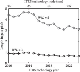
FIGURE 64.1  The length of the interconnect whose energy dissipation is equal to that of a CMOS inverter for two sizes of the inverter: (i) W/L = 1 (minimum-sized inverter) and (ii) W/L = 5 (5× the minimum-sized inverter). (Taken from S. Rakheja and A. Naeemi, Performance, energy-per-bit, and circuit size limits of post-CMOS logic circuits–Modeling, analysis and comparison with CMOS logic, in International Interconnect Technology Conference (IITC), Dresden, 2011. Copyright © IEEE 2012, with permission.)

Another challenge associated with interconnects is their growing resistivity to dimensional scaling. Owing to the enhanced electron scatterings with the grain boundaries and sidewalls in the interconnect, the material resistivity of Cu has gone up consistently with dimensional scaling. The data from the ITRS show an enhancement of Cu resistivity from 4.08 to 14.06 µΩ cm as the technology scales from 45 nm in the year 2010 to 7.5 nm by the year 2024 [8]. This increase in resistivity has enhanced the disparity in the delays of the transistors and on-chip wires. There are two metrics that capture the interconnect challenge in gigascale integration very effectively. The signal-drive distance (SDD) is the distance that a signal can travel through the interconnect in one-gate delay without using a buffer. The other metric, clock locality (CL), is the number of gate delays in a oneclock cycle and dictates how far a signal can reach on the chip without the use of a synchronization register. Owing to the degradation in the speed of interconnects, both SDD and CL show no improvement or rather a degradation with dimensional scaling as plotted in Figure 64.2.

To sustain Moore’s Law beyond the 2024 technology node, less power-hungry computational systems are required. In particular, systems that use state variables other than electronic charge may introduce a paradigm shift and open up a new scaling path [5]. An overview of the potentials and limitations of various novel state variables for beyond-CMOS computation is given in Ref. [9]. In this chapter, we consider only electron spin as the state variable for post-CMOS computation, particularly because it is one of the most studied state variables and has the potential to offer nonvolatile operation with enhanced functionality [10]. Most of the current research is focused on spin-based devices [11, 12 and 13], while not much research has been conducted so far in interconnects for spin devices. The quintessential purpose of interconnects is communication of information between various devices on the microprocessor. Hence, an analysis of the interconnection aspects early on is necessary to quantify the advantages, limitations, and opportunities of the spintronic logic. A preliminary analysis of the interconnect limits in spintronic technology, conducted in Refs. [14,15], shows that interconnects will continue to be a major bottleneck even in spintronic technology.

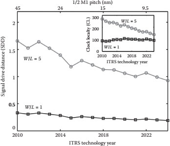
FIGURE 64.2  The signal-drive distance normalized to the gate pitch versus ITRS technology year for two inverter sizes: W/L = 1 (minimum-sized inverter) and W/L = 5 (5× the minimum-sized inverter). The inset plot shows clock locality normalized to the gate pitch versus the ITRS technology year.

The remainder of the chapter is organized as follows. First, the reference CMOS circuit that is used for comparison with the spintronic circuit is introduced. The closed-form models for the delay and the energy dissipation of the CMOS circuit are explained. The second part of the chapter introduces the all-spin logic (ASL) circuit in which graphene nanoribbons (GNRs) will be used as the channel/interconnect material of choice. Without delving into the rich physics of graphene, only the physical models of transport parameters relevant for the work in this chapter will be discussed. This part of the chapter also includes a discussion on the nanomagnets in the ASL circuit that serve as digital capacitors in the spin domain. The nanomagnets add to the overall delay and the energy consumption of ASL circuits; hence, the treatment in this chapter will be incomplete without considering the nanomagnet overhead in the spin circuit. The fourth part of the chapter is devoted to a comparison of the electrical and spintronic circuits at the 2024 technology node, which corresponds to an MFS of 7.5 nm as per the ITRS. Finally, the conclusions and outlook are provided in the last part of the chapter.

64.2  CMOS CIRCUIT

The reference CMOS circuit used for further analysis is shown in Figure 64.3. The interconnect in the CMOS circuit is implemented with Cu/low-κ and has a length L. The interconnect is driven by a CMOS driver with channel width to the length ratio denoted by W/L. The CMOS load is sized equally as the driver. The CMOS driver/load has a p-FET width double that of the n-FET to match the ON resistance of the devices. The equivalent circuit diagram is also shown in Figure 64.3, where the interconnect is represented by a distributed resistance–capacitance (r_wc_w) network. The source resistance and capacitance are denoted as R_s and C_s, respectively. The load capacitance is denoted as C_L.

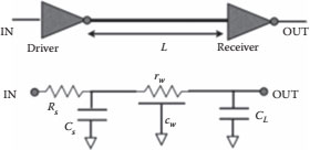
FIGURE 64.3  The schematic of the CMOS system with a CMOS driver, an interconnect, and a CMOS load (top). The equivalent circuit representation of the CMOS system (bottom).

Using the Elmore delay formula, the net delay of the circuit in Figure 64.3 can be expressed as [16]

$t_{CMOS}=0.69R_s(C_s+C_L)+0.69(R_s{c}_w+r_w{C}_L)L+0.38r_w{c}_w{L}^2.$

(64.1)

The various symbols used in Equation 64.1 and their meanings are given inTable 64.1. To evaluate the per-unit-length resistance of the interconnects, the impact of line-edge roughness and scatterings (collectively termed as “size effects”) is also considered. The grain-boundary reflectivity for Cu wires is taken to be 0.3, while the sidewall specularity parameter is selected as 0.2;^* the lineedge roughness is taken to be 40% of the interconnect width. From Table 64.1, it can be seen that the resistance per unit length of the Cu interconnect in the presence of size effects is 8× more than that of bulk Cu with the same aspect ratio and at the same technology node.

The energy dissipation of the CMOS circuit is given by the charging/discharging of all capacitances at the output node. Mathematically, this is expressed as

TABLE 64.1
Values of the Resistance and the Capacitance of Devices and Interconnects to Evaluate the Delay of the CMOS Circuit at the 2024 Technology Node

Symbol	Meaning	Value
W	Width = 1/2 M1 pitch	7.5 nm
VDD	Supply voltage	0.6 V
IDSAT	Saturation current of minimum-sized n-FET	2170 µA/µm
Rs	On-resistance of minimum-sized inverter—VDD/(IDSAT × W)	37 kΩ
Cs	Parasitic capacitance of minimum-sized inverter	6.3 aF
CL	Load capacitance of minimum-sized inverter	6.3 aF
cw	Per-unit-length capacitance of local-level M1	1.2 pF/cm
AR	Aspect ratio of interconnect = Height/Width	2.1
H	Height of the interconnect	15 nm
rw	Per-unit-length resistance of local-level M1	1.21 × 107 Ω/cm
Source:  International Technology Roadmap for Semiconductors (ITRS), 2009. Semiconductor Industry Assoc., 2009.

$E_{COMS}=\frac{1}{2}(C_s+C_L+c_{w}L)v_{DD}^2.$

(64.2)

The energy dissipation of the CMOS circuit increases linearly with the interconnect length. Hence, the energy consumption in the interconnect quickly surpasses that of the source and the load particularly when the devices are small.

Only short, local interconnects up to 100 gate pitches are considered in this analysis. The gate pitch at the 7.5 nm node is 140 nm evaluated from the ITRS by assuming an average of four transistors per gate.

64.3  ASL CIRCUIT

The ASL circuit belongs to the category of spin circuits in which the input and output are in the electrical domain, while the processing within the circuit happens in the spin domain. There are a few other notable spin-based circuits that also fall into the same category: the magnetic-tunnel junctions (MTJs) [18], the Datta–Das spin modulator [12], and the spin-FET [13]. The important feature that distinguishes all the above-mentioned devices from those in which the I/Os are also in the spin domain, such as the spin-wave bus (SWB) [19,20,21] and the magnetic quantum cellular automata (MQCA) [22], is that the former category of devices are amenable to scaling. In essence, when the footprint of the ASL circuit is reduced, the requirement on the electrical current needed to switch the magnetization of the nanomagnet devices also goes down.

While there have been several modifications to the originally proposed ASL circuit, we present a prototype in Figure 64.4 that we will use for further analysis.

In this circuit, an electrical current I_elec is used to pump spin-polarized electrons through the nanomagnet and a highly resistive tunnel barrier into the interconnect. A pure spin-diffusion current flow is set up in the interconnect; as it flows through the nonmagnetic interconnect, the amplitude of the spin-diffusion current goes down exponentially because of the finite spin flipping processes occurring within the interconnect. Finally, only a small fraction of the initially injected spin current reaches the nanomagnet receiver; depending upon the polarity of the spin current relative to that of the nanomagnet magnetization, the nanomagnet magnetization may undergo spin precession and may finally change its orientation by 180°. This is the commonly known spin-torque effect also utilized in implementing the spin-transfer torque (STT) memories. The net delay of the ASL circuit has two components: nanomagnet switching time constant (τ_mag) and the diffusion time constant of the interconnect (τ_DIFF). These individual components are discussed in detail in the next subsections. The main component of the energy dissipation of the ASL circuit is due to the ohmic heat generated along the path of the current flow. In the ASL circuit, the electrical current flows only between the terminals labeled C1T and C2T in Figure 64.4, while in the interconnect connecting the transmitter and the receiver terminals, there is no net addition of charge. The resistance along the path of the current flow is the sum of the contact resistances and the interconnect resistance sandwiched between the C1T and C2T terminals. Since the ASL circuit employs highly resistive tunnel barriers to enhance the efficiency of spin injection, the net resistance is dominated by the contacts.The energy dissipation of the ASL circuit is mathematically given as

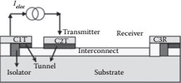
FIGURE 64.4  A representation of the ASL device proposed in Ref. [11]. An electric current pumps spinpolarized electrons through a highly resistive barrier into the interconnect. The receiver has an ohmic contact with the interconnect.

$E_{ASL}=I_{elec}^2{R}_{tx}\text{Δ}t,$

(64.3a)

$I_{elec}>\text{ς}\frac{I_{spin,thres}}{\text{η}},$

(64.3b)

where R_tx is the net resistance in the path of the current flow, and Δt is the pulse width of the electric current set to a value greater than the delay of the spin circuit. The inequality in Equation 64.3b must be satisfied to ensure that the amplitude of the spin current reaching the receiver terminal is more than the threshold current needed to toggle it. The factor ζ is called the overdrive at the receiver nanomagnet, and it is given as the ratio of the spin current actually available at the receiver to toggle it and its spin threshold current. The factor η is called the spin injection and transport efficiency (SITE), and it includes losses in the spin signal occurring while (i) injection through the tunnel barrier and (ii) the flow of the spin current through the interconnect because of the spontaneous spin flipping processes present in the nonmagnetic interconnect.

64.3.1  NANOMAGNET DYNAMICS

Spin torque refers to the phenomenon in which a pure spin current can rotate the magnetization of a nanomagnet. The component of the spin angular momentum transverse to the nanomagnet’s moment is absorbed by the nanomagnet. If the nanomagnet responds as a single domain, the magnetic moment of the nanomagnet may begin to rotate. To understand the dynamics of the nanomagnet, the effect of various torques acting on the nanomagnet must be considered. The various torques include the torques due to an applied magnetic field, magnetic anisotropies, and the intrinsic damping in the nanomagnet.

In this study, the nanomagnet is assumed to be an elliptical body shown in Figure 64.5. The magnetization is assumed to lie in the y–z plane. The shape anisotropy energy of the nanomagnet is given as

$E_{SHA}=\frac{{\text{μ}}_0}{2}{M}_S^2\Omega (N_{d,zz}{\cos }^2\text{θ}(t)+N_{d,yy}{\sin }^2\text{θ}(t)),$

(64.4)

where µ₀ is the free-space permeability, M_s is the saturation magnetization of the nanomagnet, Ω is the nanomagnet volume, θ(t) is the angle subtended by the magnetization along the easy axis (EA) at time t, and N_d,zz and N_d,yy are the demagnetization coefficients along the z- and y-axes, respectively. For θ = 0 and π, E_SHA is minimized. Hence, the axis corresponding to θ = 0 and π (z-axis in Figure 64.5) is called the EA. The axis perpendicular to the EA is called the hard axis (HA).

The dynamics of the nanomagnet under the presence of various torques due to the shape anisotropy, spin torque, and external magnetic field can be obtained by solving the Landau–Lifshitz–Gilbert (LLG) equation [24,25]. An analytical expression of the switching time of the nanomagnet under a pure spin torque as obtained in Ref. [26] is presented here:

$\begin{array}{lll}{\text{τ}}_{mag}\hfill & =\hfill & -\frac{1+{\text{α}}^2}{2\text{γα}{B}_0}{\text{μ}}_0{M}_S\Omega \frac{m}{m^2-1}\left(m\ln \left(\frac{1-m\cos v}{1+m\cos v}\right)-\ln \left(\frac{1-\cos \text{γ}}{1+\cos \text{γ}}\right)\right),\hfill \\ B_0\hfill & =\hfill & \frac{{\text{μ}}_0}{2}{M}_S^2\Omega (N_{d,zz}-N_{d,yy}),\hfill \end{array}$

(64.5)

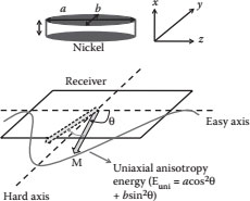
FIGURE 64.5  The top figure shows the elliptical nanomagnet with the coordinate axes. The bottom figure is the shape anisotropy energy landscape of the nanomagnet. (Taken from S. Rakheja and A. Naeemi, Interconnect analysis in spin-torque devices: Performance modeling, optimal repeater insertion, and circuitsize limits, presented at the International Symposium on Quality Electronic Design, Santa Clara, 2012. Copyright © IEEE 2012, with permission.)

where α is the dimensionless phenomenological Gilbert damping constant; γ is the gyromagnetic ratio for electrons; m = 2αB₀/s, where s = h/(4πe)ηI_elec is the spin angular momentum deposition per unit time, and the angle ν is the initial deviation of the nanomagnet magnetization from its EA. Typically, thermal fluctuations will make the magnetization deviate slightly from EA such that ν is never perfectly zero or π. However, if ν were exactly zero or π, the spin torque could never rotate the magnet. That is, for angle ν = 0/π, τ_mag → ∞, and as such these angles are also referred to as “stagnation points” in the energy landscape of the nanomagnet. The material and design parameters chosen for the nanomagnet are given in Table 64.2. For the size of the nanomagnet considered in this analysis, the thermal stability of the nanomagnet is 3k_BT, which corresponds to a spin threshold current of 0.75 µA.

Using the parameters in the Table 64.2, the switching time of the nanomagnet as a function of the initial orientation ν is plotted in Figure 64.6. The nanomagnet switching time is large for a small value of ν; this means that it is difficult for a pure spin current to induce a torque on the nanomagnet if the nanomagnet is aligned close to the EA. However, as the nanomagnet magnetization moves closer to the HA, it becomes easier for the spin current to rotate the nanomagnet magnetization. Hence, two specific kinds of switching schemes have been discussed in ASL. The first, called the full-spin torque (FST) switching, utilizes only pure spin currents to rotate the nanomagnet. For FST switching, the initial orientation of the nanomagnet is ν → 0. In a different scheme, one can use Bennett clocking to align the nanomagnet along its HA (ν → π/2); hence, the input electrical current is now required to only tip the nanomagnet toward one of its stable states. This is called the mixed-mode (MM) switching. There are, of course, issues related to the thermal stability of the nanomagnet and energy dissipation in the clocking scheme required for the MM switching of the nanomagnet. However, in principle, MM switching would be much faster compared to the FST switching. A novel proposal to use the nanomagnet in the MM switching mode is discussed in Refs. [26,27] in which a voltage-generated stress in a multiferroic magnet consisting of a magnetostrictive layer (nickel) and a piezoelectric layer is used to rotate the nanomagnet to ν ~ π/2. In another MM scheme in Ref. [11], it is discussed that applying a voltage to a fixed magnetic layer in contact with the output magnetic layer through the spacer layer can help accumulate spins in the direction of the fixed layer; these spins can then apply a spin torque on the output magnet and rotate it to its HA. However, the details and issues related to these approaches are beyond the scope of this chapter.

TABLE 64.2
Material and Design Parameters for the Nanomagnet (Nickel)

Parameter	Value
Major axis dimension of the nanomagnet	16.5 nm
Minor axis dimension of the nanomagnet	10 nm
Thickness of the nanomagnet	5 nm
Saturation magnetization, Ms	3.93 × 105 A/m
Damping coefficient, α	0.01
Uniaxial shape anisotropy	3 kBT
Threshold current of the receiver, Ispin,thres	0.75 µA
Source:  Taken from S. Rakheja and A. Naeemi, Interconnect analysis in spin-torque devices: Performance modeling, optimal repeater insertion, and circuit-size limits, presented at the International Symposium on Quality Electronic Design, Santa Clara, 2012. Copyright © IEEE 2012, with permission.

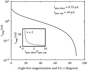
FIGURE 64.6  Switching time of the nanomagnet versus the angle ν. The inset plot shows the impact of the input spin current on nanomagnet switching time.

The inset plot of Figure 64.6 shows the impact of increasing the input spin current to induce spintorque-assisted switching of the nanomagnet. The horizontal x-axis in the inset plot is the factor 1/ζ as in Equation 64.3b. As the input current increases, the overdrive of the spin current available at the nanomagnet increases, making it easier for the spin current to switch the nanomagnet magnetization. However, the improvement in the nanomagnet delay saturates with an increase in the input spin current. An optimal ζ can be determined such that the energy dissipation of the nanomagnet is minimized. As ζ increases, the input electrical current increases, which increases the I²R heating the circuit. However, because the nanomagnet toggles faster with an increase in ζ, the landscape of the energy dissipated in the nanomagnet versus ζ will exhibit a minimum energy point.

64.3.2  INTERCONNECT DYNAMICS

The interconnect in the ASL circuit can be implemented using a variety of materials. Metals like Cu and Al have an established technology and, therefore, from a fabrication perspective, would be a good choice. In addition, their resistivity values could be comparable to that of the injecting nanomagnet. This can help to overcome the well-known “conductivity mismatch” issue in spinbased devices [28,29]. However, the spin-relaxation length in metals is usually limited to only a few 100s of nanometers [30,31]. Semiconductors such as Si and GaAs may also be good choices for implementing interconnects in the ASL circuit. However, appreciable spin injection in semiconductors could be an issue [32]. Carbon-based material graphene has a very rich physics that provides it superior electrical and spintronic characteristics desirable of interconnects in the ASL circuit. Graphene, owing to its large electron mean free path (MFP), may support a fast spin-current transport through it. Further, owing to its low atomic number, graphene also has a reduced spin–orbit coupling (SOC) lending it long spin-relaxation lengths [33]. In this work, the focus will be on narrow patterned GNRs as the interconnect material of choice in the ASL circuit.

Graphene can support a quasi-ballistic transport of electron spins through it. In the steady state, the flux of the electron spins through the interconnect is given as [34]

$J_s=\frac{D}{L}\frac{s(0)}{1+\frac{D}{L}\frac{1}{v_f}},$

(64.6)

where s(0) is the electron spin concentration in 1/cm at the beginning of the interconnect, D is the diffusivity of carriers in the interconnect in cm²/s, L is the interconnect length in cm, and ν_f is the Fermi velocity of carriers in cm/s. The steady-state carrier concentration in the interconnect is given by a linear profile as

$s(z)=s(0)\left(1-\frac{z}{L}\right)+\frac{s(L)}{L}.$

(64.7)

The time constant of spin diffusion through the interconnect can be given as

${\text{τ}}_{DIFF}=\frac{{\displaystyle {\displaystyle \underset{0}{\overset{L}{\int }}}s(z)dz}}{J_s}.$

(64.8)

Using Equations 64.6 through 64.8, τ_DIFF can be simplified as

${\text{τ}}_{DIFF}=\frac{L^2}{2D}+\frac{L}{v_f}.$

(64.9)

The first component in Equation 64.9 is the diffusive time constant and the second component is the ballistic time constant. From Equation 64.9, it can also be seen that the speed of the spin-diffusion interconnects is governed by the material parameters: diffusion coefficient, D, and Fermi velocity, v_f. The delay of spin interconnects increases quadratically with their length much like the intrinsic delay of electrical interconnects.

Next, the physical models of the electron diffusion coefficient in bulk and 1D graphene are presented.

64.3.2.1  Diffusion Coefficient in GNRs

In 2D graphene, the electron diffusion coefficient, D, is related to the electron MFP, λ, according to D = 1/2λv_f. The electron MFP in 2D graphene is obtained by taking contributions to electron scatterings from the intrinsic phonons in graphene (acoustic and optical), and extrinsic sources arising from the substrate underneath the graphene sheet. For a suspended graphene sheet, the electron MFP can be as high as 1–1.2 µm as obtained experimentally in [35,36]. However, when deposited or grown epitaxially on a substrate, the electron MFP in graphene is limited to only a few hundred nanometers or even lower [37]. Hence, the substrate can easily limit the best-possible diffusion coefficient in graphene. Table 64.3 shows the impurity concentration and remote-phonon-limited MFP for various substrates for an electron concentration of 10¹² cm⁻² in the graphene sheet.

Using the data from Table 64.3, the electron diffusion coefficient in 2D graphene is obtained as a function of carrier concentration and is plotted in Figure 64.7 for various substrates at RT. The best-case diffusion coefficient for graphene is obtained in the case of h-BN substrate because of the nearly perfect lattice matching of h-BN with graphene, which can significantly reduce the surface roughness of h-BN. For an electron concentration, N_s, in the range (1–5) × 10¹² cm⁻², the diffusion coefficient of electrons in graphene on h-BN lies between 1000 and 1200 cm²/s. This corresponds to an electron MFP of 250–300 nm. For graphene SiO₂, the diffusion coefficient is 408 cm²/s for N_s = 10¹² cm⁻²; this corresponds to an electron MFP of 102 nm.

However, once graphene is patterned into narrow ribbons for use as interconnects and devices, there occurs a quantization of electron energies along the width of the graphene. The energy-dispersion relation of GNRs is given as [41]

$E=h{v}_f\sqrt{k_{\parallel }^2+k_{\perp }^2},$

(64.10)

where k_|| is the wave vector along the length of the ribbon and k_⊥ is the wave vector along the ribbon width and is quantized according to

$k_{\perp }=\frac{\text{π}}{W}\left|m+\text{β}\right|,$

(64.11)

where W is the ribbon width, and β = 0 for metallic ribbons and 1/3 for semiconducting ribbons. Experiments have confirmed that all narrow ribbons are semiconducting and that the orientation effects are all washed out for narrow ribbons [42]. Hence, we choose β = 1/3 for all further analysis. The low-field 1D conductivity according to Landauer’s formalism is given as

${\text{σ}}_{1D}=-\frac{2e^2}{h}{\displaystyle {\displaystyle \sum _m}{\displaystyle {\displaystyle \underset{E_{sub,m}}{\overset{\infty }{\int }}}{\lambda }_m(E)\frac{\partial f_{FD}(E)}{\partial E}dE}},$

(64.12)

TABLE 64.3
Concentration of Charged Impurities and the Remote-Phonon-Limited MFP at RT for an Electron Concentration, N_s = 10¹² cm⁻²

Substrate	Charged-Impurity Concentration (cm−2)	Remote-Phonon-Limited MFP at RT for Ns = 1012 cm−2 (nm)
SiO2	(1.3–1.8) × 1011	195
SiC	(0.6–1) × 1011	575
SrTiO3 (STO)	(0.7–1.3) ×1011	53
HfO2	—	35
h-BN	<7 × 1010	920
Source: Data taken from F. Giannazzo et al., Nano Letters, 11, 4612–4618, 2011; C. Dean, et al., Nature Nanotechnology, 5, 722–726, 2010; and V. Perebeinos and P. Avouris, Physical Review B, 81, 2010.

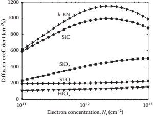
FIGURE 64.7  Diffusion coefficient in graphene on various substrates versus electron concentration at RT.

where e is the electron charge, h is the Planck’s constant, f_FD(E) is the Fermi–Dirac statistics, and λ_m(E) is the electron MFP in the mth conduction channel in the GNR. The summation in Equation 64.12 runs over all the conduction channels in the GNR. The electron diffusion coefficient is then obtained using Equation 64.12 in conjunction with Einstein’s relationship and is mathematically expressed as

$D=\frac{\text{σ}}{e^2\partial n_{1D}/\partial E_f},$

(64.13)

where n_1D is the 1D carrier concentration in the GNR and is obtained by the convolution of the density of states with the Fermi–Dirac statistics in the energy space. The electron MFP, λ_m(E), is obtained by using Mattheissen’s rule for the edge-scattering limited MFP, ${\lambda }_m^{edge}(E)$, and the substrate-limited MFP, λ_sub. Patterning graphene into narrow ribbons renders its edges rough and can introduce additional scattering of electrons. Indeed, experiments have shown that a 2.5 nm wide GNR deposited on SiO₂ has an electron mobility as low as 200 cm²/Vs at RT, which corresponds to an electron MFP of 12 nm [43]. This value of electron MFP is significantly lower than a value of ~100 nm for a wide graphene flake on SiO₂.

The MFP associated with the diffusive scatterings at the edges is a function of the scattering probability at the edges (P_GNR) and the average distance that the electrons move along the length of the ribbon before hitting one of the edges. Mathematically, the edge-scattering MFP is given as [41]

${\lambda }_m^{edge}(E)=\frac{1}{P_{GNR}}\frac{k_{\parallel }}{k_{\perp }}W=\frac{W}{P_{GNR}}\sqrt{{\left(\frac{E}{E_{sub,m}}\right)}^2-1},$

(64.14)

where E_sub,m is the minimum of the mth sub-band energy. The effective MFP of electrons in GNR on various substrates is plotted as a function of the GNR width for P_GNR = 0.2 in Figure 64.8. Two values for the Fermi-energy shift, E_f, in graphene have been considered. Experiments have shown that because of a work-function difference in the substrate and graphene sheet, the Fermi energy in the graphene sheet is usually positive. Values of E_f = 0.2 eV and 0.4 eV have been experimentally obtained [44,45]. For all GNR widths, the effective MFP increases with an increase in the Fermi energy and substrate-limited MFP. The electron MFP for a suspended wide graphene sheet measured by Bolotin and coworkers in 2008 was 1.2 µm for an electron concentration of 2 × 10¹¹ cm⁻² [35]. Even when the substrate-limited MFP is as high as 1.2 µm,^* there is more than a 10× drop in the effective electron MFP of a 10-nm-wide GNR with a 20% edge-scattering probability. For sub-10 nm GNR widths, the effective electron MFP will be limited to only a few tens of nm, particularly for substrates like SiO₂ for which λ_sub < 100 nm.

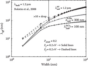
FIGURE 64.8  The effective MFP of electrons in GNR as a function of its width. The substrate-limited MFP for h-BN is taken to be 300 nm, while that for SiO₂ is 100 nm.

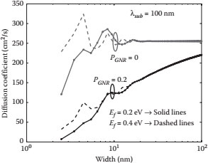
FIGURE 64.9  Electron diffusion coefficient in GNR versus the GNR width for the SiO₂ substrate. Various values of the Fermi-energy shift, E_f, and the edge-scattering coefficient, P_GNR, have been selected for simulation.

The electron diffusion coefficient in the GNR on SiO₂ as a function of the GNR width is shown in Figure 64.9 for various values of P_GNR and E_f. The substrate is chosen to be SiO₂ as most experiments in graphene spin valves have been conducted for graphene deposited on SiO₂; other substrates have been far less explored for potential applications in spintronics. The diffusion coefficient improves with an increase in the GNR width and a reduction in edge roughness (characterized by a lower value of P_GNR). At a GNR width of 7.5 nm and a Fermi-energy shift E_f = 0.2 eV, the electron diffusion coefficient is 280 cm²/s in the absence of edge scatterings (P_GNR = 0). However, for P_GNR = 0.2, the electron diffusion coefficient drops to 105 cm²/s if all other parameters are the same.

64.3.2.2  Spin-Relaxation Length in Graphene

Unlike electrical current, spin current is not a conserved quantity. That is to say, the amplitude of the spin current decays in an exponential fashion as it moves through the interconnect. This behavior of the spin current is captured through the spin-relaxation time (τ_s) and the spin-relaxation length (L_s); these parameters are related through the diffusion coefficient as L_s = (Dτ_s)^0.5. The principal cause of spin relaxation in materials is the presence of a finite atomic SOC in materials that leads to an interaction between the spin and the orbital angular momentum of electrons. The atomic SOC rises sharply with the atomic number (~Z ⁴); hence, the atomic SOC in graphene is rather weak due to its low atomic number (Z = 6). However, the presence of ripples in graphene creates an additional SOC, which is at least 20× in strength compared to the atomic SOC [33,46,47]. In addition, extrinsic sources such as remote polar phonons and impurities in the substrate on which graphene is grown or deposited can also enhance SOC and lead to a faster spin relaxation.

In Table 64.4, various SOCs in graphene from theoretical estimates are provided. From theoretical studies in Ref. [33], it was found that the spin-relaxation length in pristine graphene could be as high as 15–20 µm. Further, when (K_fλ)² ≫ 1, the spin-relaxation time is insensitive to the momentum-relaxation time in graphene. Here, K_f is the Fermi wave-vector. This is the characteristic D’yakonov–Perel’ (DP) spin-relaxation mechanism. In the other extreme, when (K_fλ)² ≪1, the spin-relaxation time is proportional to the momentum-relaxation time. This is commonly referred to as the Elliott–Yafet (EY) spin-relaxation mechanism [48]. Hence, depending upon the product of the Fermi wave vector and the electron MFP in graphene, the spin-relaxation mechanism in graphene could change from EY to DP. Recent experiments on spin relaxation in graphene show a limited spin-relaxation length of 2–3 µm at RT [49, 50, 51, 52 and 53]. Further, the nature of the spin-relaxation mechanism in Ref. [54] is EY-type, while for the experiment in Ref. [55], the nature of spin-relaxation mechanism is DP. One of the reasons for the controversial experimental results and theoretical estimates is that in the experimental samples there is an appreciable concentration of adatoms. These adatoms hybridize with the carbon atoms of graphene and modify the otherwise sp² bonding of graphene to sp³ bonding. The strength of the SOC associated with these adatoms could be as high as a few meV [56]. Further, the nature of the spin relaxation due to adatoms could also change from EY to DP, depending upon environmental factors such as the electron concentration, adatom concentration, and ambient temperature. For a thorough theoretical investigation of the spin relaxation mediated by the random Rashba field (RRF) of adatoms in graphene, see Ref. [57].

TABLE 64.4
Various SOCs in Graphene

Coupling Constant	Value (eV)	Spin-Relaxation Time, τs	Reference
Δsoint (atomic)	8.6 × 10−7	18 µs	[33]
Δsocurv (curvature)	1.7 × 10−5	0.28 µs	[33]
Δsosub(substrate SiO2) (Nimp = 4 × 1011 cm−2)	7.24 × 10−8	0.6 ms	[56]
Δsosub(substrate SiO2) (Nimp = 4 × 1012 cm−2)	2.17 × 10−6	6 µs	[56]
Note:    Nimp denotes the impurity concentration. The curvature-induced coupling depends on the ripple radius, which has been assumed to be between 50 and 100 nm. The value of substrate-induced τs is quoted for a Fermi energy of 0.1 eV. All values are at RT.

In the case of GNRs, there is an additional SOC introduced by the edge states. However, for the case where (K_fλ)² ≫ 1, the spin-relaxation length will not be much different from that in the bulk assuming that the effective SOC is equal to the ripple-induced SOC; for this regime, the spin-relaxation length will only be slightly sensitive to the edge-scattering coefficient.

In this analysis, simulations are conducted for the two values of spin-relaxation length: (i) L_s = 15 µm (best-case) and (ii) L_s = 2 µm (experimental).

64.3.2.3  Spin Injection and Transport Efficiency

Spin injection and transport efficiency (SITE) in the ASL circuit gives the amount of spin current reaching the receiver per unit of input electrical current in the system. The mathematical details to obtain SITE in the ASL circuit will not be presented. Interested readers can refer to Ref. [29]. Briefly stated, the method consists of solving the spin quasi-chemical potential in various regions of the circuit and applying appropriate boundary conditions. At the interfaces, the spin current is balanced, while a discontinuity in the spin quasi-chemical potential is created at the interface in the presence of tunnel barriers. The spin quasi-chemical potential equation is a second-order ODE given as

$\frac{{\text{d}}^2{\text{μ}}_s}{\text{d}{x}^2}=\frac{{\text{μ}}_s}{L_S^2},$

(64.15)

where µ_s is the difference in the chemical potential of the up-spin and down-spin carriers at any given location in the ASL circuit. The spin current for a nanomagnet is the sum of the current generated due to spatial variation in µ_s and also due to an applied bias. For a nonmagnetic interconnect, the spin current arises only because of the spatial variation in µ_s (also termed as “spin accumulation”), while an applied bias is insufficient by itself to generate a spin current in a nonmagnetic interconnect.

In Figure 64.10, SITE is plotted as a function of the interconnect length for a 7.5-nm-wide GNR for L_s = 2 µm and 15 µm for various values of P_GNR. It can be seen from this figure that SITE degrades rapidly with an increase in the interconnect length, particularly for a short L_s and a greater edge roughness. For example, for P_GNR = 0.2 and L_s = 2 µm, SITE is 0.135 for L = 1 µm (point “a” in Figure 64.10), and SITE degrades to 1.1 × 10⁻³ for L = 10 µm (point “b” in Figure 64.10). For L_s = 15 µm, the degradation in SITE is from 0.144 to 1.8 × 10⁻² as L increases from 1 to 10 µm for P_GNR = 0.2. This degradation in SITE will necessitate pumping in more electrical current in the transmitter of the ASL so that an appreciable spin current reaches the receiver. This translates to a rapid increase in the energy dissipation of the ASL circuit as will be shown in the next section.

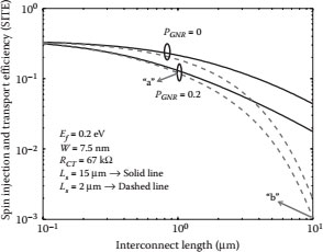
FIGURE 64.10  SITE for an ASL circuit with a 7.5-nm-wide GNR interconnect versus the interconnect length. R_CT denotes the total contact resistance at the transmitter. Two values of the spin-relaxation length in the GNR are considered. A 2 µm value of L_s is from experiments, while 15 µm is from theoretical estimates (best-case value).

64.4  COMPARISON OF ELECTRICAL AND SPINTRONIC CIRCUITS

In Figure 64.11, the delays of the spintronic and CMOS systems are plotted as a function of the interconnect length at the 7.5 nm technology node. For the CMOS system, the delay is computed using Equation 64.1. For the spin system, the delay is computed using Equations 64.5 and 64.9 to account for both the nanomagnet switching and the interconnect switching. To be able to compute the delay of the nanomagnet, the overdrive at the nanomagnet must be known. As illustrated in Figure 64.6, the nanomagnet becomes particularly sluggish if the spin current available to switch the nanomagnet is not sufficiently higher than its threshold current. For the simulation of the delay, an overdrive of 10× is assumed at all interconnect lengths. That is, ζ = 10. However, the input current can be optimized to yield a minimum energy dissipation of the ASL circuit for the given interconnect dimensions.

From Figure 64.11, it can be seen that even without considering the overhead of the nanomagnet switching, the delay of the ASL circuit governed only by the native interconnect delay increases more rapidly with the interconnect length when compared with the delay of the CMOS system. In fact, even short, local GNR spin interconnects longer than one or two gate pitches at the 7.5 nm interconnect technology node have a delay higher than that of the CMOS system. Further, the nanomagnet switching time for FST mode is 9.7 ns for a 10× overdrive; hence, in the FST mode, the dominant time constant is that of the receiver nanomagnet. The ASL circuit is orders of magnitude slower than the CMOS circuit. The switching time of the receiver nanomagnet can be lowered significantly by utilizing the MM switching mode. However, in this case, as the overall time constant is dominated by the spin interconnect, the ASL circuit delay increases with the interconnect length, and it is still much slower compared to the CMOS circuit.

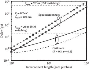
FIGURE 64.11  Delay versus interconnect length for both the ASL and CMOS circuits. For the CMOS circuit, R denotes the grain-boundary reflectivity, while p denotes the sidewall specularity. No line-edge roughness has been considered. The dashed horizontal lines correspond to the intrinsic delay of nanomagnet switching in both the FST and MM switching modes.

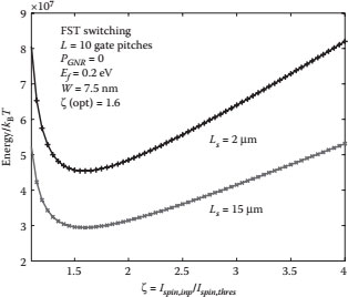
FIGURE 64.12  Energy of the ASL circuit versus the overdrive at the receiver nanomagnet. The optimal value of the overdrive in the FST switching mode is 1.6, independent of the interconnect length and the spin-relaxation length in the interconnect.

As discussed in Section 64.3.1, the value of the overdrive at the receiver nanomagnet can be optimized to minimize the energy dissipation of the ASL circuit. In Figure 64.12, the total energy dissipation of the ASL circuit with the FST mode of nanomagnet switching is shown as a function of the overdrive factor, ζ. This optimal energy point depends only upon the nanomagnet dynamics. For the material and design parameters chosen, the optimal ζ = 1.6 for the FST mode of switching. In the MM switching mode, the delay of the nanomagnet decreases very gradually with an increase in ζ, while the Joule heating term I²R grows quadratically with ζ. Hence, in the MM switching mode, the optimal value of ζ that minimizes the energy dissipation is very close to unity.

InFigure 64.13, the energy dissipation of the ASL circuit is plotted as a function of the interconnect length using the optimal value of ζ. The total transmitter-side resistance is taken to be 67 kΩ.^* It can be seen that for the simulation parameters selected, the energy dissipation of the ASL circuit is higher than that of the CMOS circuit. Further, owing to the rapid increase in the energy dissipation of the ASL circuit with interconnect length, the disparity in the energy dissipation of ASL and CMOS circuits grows with an increase in length.

The simulation results presented here conclusively show that interconnects will continue to be a major challenge even in spintronics technology. Hence, spin circuits that require shorter interconnects either by scaling the footprint of devices more aggressively or by using smart architectures with fewer gates to implement a function will be important to make spintronic technology competitive with respect to the charge-based technology. In addition, parallelism that can mask the delay of interconnects will also be favorable to the spintronic technology. It is quite likely that short, local interconnects are implemented as spin interconnects while intermediate and global-level interconnects are electrical in future spin circuits.

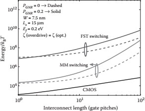
FIGURE 64.13  Energy dissipation versus the interconnect length for both the ASL and CMOS circuits. Both the FST and MM switching modes are considered for the ASL circuit.

64.5  CONCLUSIONS AND OUTLOOK

In this chapter, the limits imposed by interconnects in the ASL circuit are quantified. While for CMOS circuits it is well established that interconnects are one of the grandest challenges in gigascale integration, relatively little research has been conducted in quantifying interconnect limits in spin-based circuits.

The net delay of the ASL circuit is given by the sum of the delays of the nanomagnet and the interconnect. For the nanomagnet switching, a full-spin torque-assisted switching is much more sluggish when compared with a MM switching utilizing Bennett clocking to align the nanomagnet along its HA that utilizes spin current to only tip the nanomagnet toward one of its stable states. The interconnect delay in the ASL circuit is shown to increase quadratically with the interconnect length and varies as 1/D, where D is the spin diffusion coefficient in the interconnect. Owing to the finite spin-relaxation length in the interconnect material, the amount of spin current reaching the receiver is substantially less than the ideal case. This makes the nanomagnet sluggish particularly for interconnects longer than the spin-relaxation length. The energy dissipation of the ASL circuit is given by the Joule heating occurring along the path of the current flow, which in the case of the ASL circuit is limited to the transmitter side.

Owing to its unique and rich physics, graphene has turned out to be an interesting material for future devices in both the electrical and spin-based domains. This chapter provides physical models of the electron diffusion coefficient in narrow graphene ribbons as a function of the interconnect dimensions and the edge roughness. The spin-relaxation length in graphene could be as high as 15–20 µm if only ripple-induced SOC is considered. However, in most experiments, a limited spin-relaxation length of 2 µm is measured, illustrating the limits imposed by metallic adatoms on the spin transport through a graphene channel. Using both the optimistic and realistic values of the spin-relaxation length in graphene, SITE of the ASL circuit is obtained. It is shown that SITE degrades rapidly with an increase in the interconnect length and with an increase in the edge roughness of the GNR. SITE also drops drastically for shorter spin-relaxation lengths in the interconnect.

It is shown that both the delay and the energy dissipation of the ASL circuit do not compare well with those of its CMOS counterparts. However, by designing spin-based circuits with smarter architectures that favor shorter interconnects, it may be possible to achieve faster spin circuits while dissipating relatively low energy. Parallelism of computation may also play a significant role in lowering the overall switching time constant of the ASL circuit, thereby improving both its speed and energy dissipation.

In its quest to sustain Moore’s law for sub-10 nm nodes, the current research in nanoelectronics is rich with exploratory ideas for the next-generation switch. With this accelerated progress, one can certainly be hopeful for a new technology to emerge in the near future that would either augment or replace the current CMOS technology and establish a new scaling path for computation.

REFERENCES

1.  M. S. Bakir and J. D. Meindl, Integrated Interconnect Technologies for 3D Nanoelectronic Systems (Integrated Microsystems), 1st ed. Boston, MA: Artech House Publishers, 2008.

2.  V. V. Zhirnov et al., Limits to binary logic switch scaling—A Gedanken model, Proceedings of the IEEE, 91, 1934–1939, 2003.

3.  R. K. Cavin et al., Energy barriers, demons, and minimum energy operations of electronic devices, Fluctuation and Noise Letters, 5, 29–38, 2005.

4.  R. Cavin et al., Research directions and challenges in nanoelectronics, Journal of Nanoparticle Research, 8, 841–858, 2006.

5.  G. Bourianoff, The future of nanocomputing, Computer, 36, 44–53, 2003.

6.  N. Magen et al., Interconnect-power dissipation in a microprocessor, presented at the Proc. Int. Workshop System Level Interconnect Prediction, Paris, France, 2004.

7.  S. Rakheja and A. Naeemi, Performance, energy-per-bit, and circuit size limits of post-CMOS logic circuits–Modeling, analysis and comparison with CMOS logic, in International Interconnect Technology Conference (IITC), Dresden, 2011.

8.  International Technology Roadmap for Semiconductors (ITRS), 2009. Semiconductor Industry Assoc., 2009.

9.  K. Galatsis et al., Alternate state variables for emerging nanoelectronic devices, IEEE Trans. Nanotechnology, 8, 66–75, 2009.

10.  D. D. Awschalom and M. E. Flatte, Challenges for semiconductor spintronics, Nature Physics, 3, 153–159, 2007.

11.  B. Behin-Aein et al., Proposal for an all-spin logic device with built in memory, Nature Nanotechnology, 5, 266–270, 2010.

12.  S. Datta and B. Das, Electronic analog of the electro-optic modulator, Applied Physics Letters, 56, 665–667, 1990.

13.  S. Sughara and J. Nitta, Spin transistor electrons: An overview and outlook, Proceedings of the IEEE, 98, 2124–2154, 2010.

14.  S. Rakheja and A. Naeemi, Interconnects for novel state variables: Performance modeling and device and circuit implications, IEEE Transactions on Electron Devices, 57, 2711–2718, 2010.

15.  S. Rakheja and A. Naeemi, Modeling interconnects for post-CMOS devices and comparison with copper interconnects, IEEE Transactions on Electron Devices, 58, 1319–1328, 2011.

16.  H. B. Bakoglu, Circuits, Interconnections and Packaging for VLSI, 1 ed., Addison-Wesley, 1990.

17.  S. M. Rossnagel and T. S. Kuan, Alteration of Cu conductivity in the size effect regime, Journal of Vacuum Science & Technology B: Microelectronics and Nanometer Structures, 22, 240–247, 2004.

18.  J.-G. Zhu and C. Park, Magnetic tunnel junctions, Materials Today, 9, 36–45, 2006.

19.  A. Khitun et al., Feasibility study of logic circuits with a spin wave bus, Nanotechnology, 18, 465202 (9 pages), 2007.

20.  A. Khitun and K. L. Wang, Nano scale computational architectures with spin wave bus, Superlattices and Microstructures, 38, 184–200, 2005.

21.  A. Khitun et al., Efficiency of spin-wave bus for information transmission, Electron Devices, IEEE Transactions on, 54, 3418–3421, 2007.

22.  A. Imre et al., Majority logic gate for magnetic quantum-dot cellular automata, Science, 311, 205–208, 2006.

23.  S. Rakheja and A. Naeemi, Interconnect analysis in spin-torque devices: Performance modeling, optimal repeater insertion, and circuit-size limits, presented at the International Symposium on Quality Electronic Design, Santa Clara, 2012.

24.  J. Z. Sun et al., A three-terminal spin-torque-driven magnetic switch, Applied Physics Letters, 95, 083506, 2009.

25.  J. Z. Sun, Spin-current interaction with a monodomain magnetic body: A model study, Physical Review B, 62, 570–578, 2000.

26.   K. Roy et al., Hybrid spintronics and straintronics: A magnetic technology for ultra low power energy computing and signal processing, Applied Physics Letters, 99, 063108 (3 pages), 2011.

27.  M. Salehi-Fashmi et al., Ultra low-power straintronics with multiferroic nanomagnets: Magnetization dynamics, universal logic gates and associated energy dissipation, presented at the APS March Meeting, Boston, MA, 2012.

28.  J. Fabian et al., Semiconductor spintronics, Acta Physica Slovaca, 57, 565–907, 2007.

29.  I. Zutic et al., Spintronics: Fundamentals and applications, Reviews of Modern Physics, 76, 323–410, 2004.

30.  F. J. Jedema et al., Electrical detection of spin precession in a metallic mesoscopic spin valve, Nature, 46, 713–716, 2002.

31.  F. J. Jedema et al., Spin injection and spin accumulation in all-metal mesoscopic spin valves, Physical Review B, 2003, 085319 (16 pages), 2003.

32.  S. P. Dash et al., Electrical creation of spin polarization in silicon at room temperature, Nature, 462, 491–494, 2009.

33.  D. Hernando et al., Spin–orbit coupling in curved graphene, fullerenes, and nanotube caps, Physical Review B, 74, 155426 (15 Pages), 2006.

34.  M. Lundstrom, Fundamentals of Carrier Transport, 2nd ed. Cambridge, UK: Cambridge University Press, 2000.

35.  K. I. Bolotin et al., Ultrahigh electron mobility in suspended graphene, Solid State Communications, 146, 351–355, 2008.

36.  X. Du et al., Approaching ballistic transport in suspended graphene, Nature Nanotechnology, 3, 491–495, 2008.

37.  T. Shimizu et al., Large intrinsic energy bandgaps in annealed nanotube-derived graphene nanoribbons, Nature Nanotechnology, 6, 6, 2011.

38.  F. Giannazzo et al., Mapping the density of scattering centers limiting the electron mean free path in graphene, Nano Letters, 11, 4612–4618, 2011.

39.  C. Dean et al., Boron nitride substrate for high-quality graphene electronics, Nature Nanotechnology, 5, 722–726, 2010.

40.  V. Perebeinos and P. Avouris, Inelastic scattering and current saturation in graphene, Physical Review B, 81, 195442 (8 pages), 2010.

41.  A. Naeemi and J. D. Meindl, Compact physics-based circuit models for graphene nanoribbon interconnects, IEEE Transactions on Electron Devices, 56, 1822–1833, 2009.

42.  D. Queriloz et al., Suppression of the orientation effects on bandgap in graphene nanoribbons in the presence of edge disorder, Applied Physics Letters, 92, 042108, 2008.

43.  X. Wang et al., Room-temperature all-semiconducting sub-10-nm graphene nanoribbon field-effect transistors, Physical Review Letters, 100, 206803–206804, 2008.

44.  S. Y. Zhou et al., Substrate-induced bandgap opening in epitaxial graphene, Nature Materials, 6, 770–775, 2007.

45.  C. Berger et al., Electronic confinement and coherence in patterned epitaxial graphene, Science, 312, 1191–1196, 2006.

46.  D. Huertas-Hernando et al., Spin–orbit-mediated spin relaxation in graphene, Physical Review Letters, 103, 146801 (4 pages), 2009.

47.  D. Heurtas-Hernando et al., Spin relaxation times in disordered graphene, The European Physical Journal-Special Topics, 148, 178–181, 2007.

48.  H. Ochoa, A. H. Castro Neto, and F. Guinea, Elliot-Yafet mechanism in graphene, Applied Physics Letters, 108 (20), 206808, 2012.

49.  W. Han et al., Enhanced spin injection into graphene with MgO tunnel barriers, APS March Meeting, 35.006, 2010.

50.  W. Han et al., Electrical detection of spin precession in single layer graphene spin valves with transparent contacts, Applied Physics Letters, 94, 22109–22109–3, 2009.

51.  M. Shiraishi, M. Ohishi, R. Nouchi, N. Mitoma, T. Nozaki, T. Shinjo, and Y. Suzuki, Robustness of spin polarization in graphene-based spin valves, Advanced Functional Materials, 19(23), 3711–3716, 2009.

52.  M. Popinciuc et al., Electronic spin transport in graphene field effect transistors, Physical Review B, 80, 214427, 2009.

53.  N. Tombros et al., Electronic spin transport and spin precession in single graphene layers at room temperature, Nature, 448, 571–574, 2007.

54.  C. Jozsa et al., Linear scaling between momentum and spin scattering in graphene, Physical Review B, 80, 241403 (4 pages), 2009.

55.   W. Han and R. Kawakami, Spin relaxation in single-layer and bilayer graphene, Physical Review Letters, 107, 047207 (4 pages), 2011.

56.  C. Ertler et al., Electron spin relaxation in graphene: The role of the substrate, Physical Review B, 80, 4, 2009.

57.  P. Zhang and M. W. Wu, Electron spin relaxation in graphene with random Rashba field: Comparison of the D’yakonov–Perel’ and Elliott–Yafet-like mechanisms, New Journal of Physics, 14, 033015 (22 pages) 2012.

Notes

*.  The interface between Cu and Ta is diffusive due to a mismatch in the Fermi surfaces of the two materials. Hence, electrons in narrow and thin Cu wires suffer from diffuse scatterings at the sidewalls rendering a low value to the sidewall specularity parameter. From most experiments, the sidewall specularity was extracted between 0 and 0.2 [17].

*.  A substrate with λ_sub = 1.2 µm is referred to as an “ideal” or “air” substrate.

*.  This corresponds to approximately 1.9 conduction channels at RT for a 7.5 nm wide GNR with a Fermi-energy shift of 0.2 eV. The transmission coefficient of electrons from the contacts into the graphene channel is taken to be 0.1 for the transmitter side.