Configuration management (CM) tools like Puppet and Chef are really useful for keeping your systems in line, but what about your infrastructure? The Really Awesome New Cisco confIg Differ—or RANCID for short—is the first step in tackling this problem. In essence, RANCID is a suite of utilities that enables automatic retention of your configurations in revision control. If you have a physical infrastructure at any level, you should be working to have the same level of control as you do on your servers with your CM solution.

So that sounds good, but what problem does RANCID really solve? The core usage is to create an audit trail of software configurations and hardware information for the devices that glue servers together. The configuration of your switches, routers, and load balancers may not be changing as fast as the code in your Rails app (at least I hope not!), but it does change over time. The rate of change is usually tied to how fast your environment is either changing or expanding.

Auditing is a great first step in the automation process. You have to know where you are to get where you’re going after all! RANCID does this out of the box for devices from Cisco, Juniper, F5, and many other vendors. The audit process requires a basic installation of RANCID and configuration of a read-only user on the devices you want to monitor. The result is a current configuration automatically pulled on a regular schedule, committed to revision control, and an email detailing the changes in your inbox.

So now you’re ready to try out RANCID, but where to start? If you are a Subversion shop, you’re set—go grab the latest tarball and follow along with the Getting Started guide. Git users can grab a fork of RANCID that is patched to add git functionality. Though git isn’t natively supported by the maintainer of RANCID, I prefer git to Subversion, so that’s the codebase that I use.

Once you have RANCID installed, there are a few base configuration items that need to be set in /etc/rancid/rancid.conf (or wherever your rancid.conf was installed).

rancid.conf

RCSSYS=git
FILTER_PWDS=YES
LIST_OF_GROUPS="pdx slc ord"

Configuring RANCID to pull configs requires the username and password used to connect to each device, optionally using hostname matching. RANCID supports connecting to devices over telnet and ssh. I’m sure this goes without saying, but don’t use telnet, and don’t even enable it on the devices! Some devices support key-based authentication (like Juniper and F5) and do not require passwords. In this case, RANCID will use the ssh key if one has been configured for the ranice user, and RANCID is configured to connect via ssh. Otherwise you configure passwords in the .cloginrc file, which can be found in the rancid user’s home directory. Here is an example:

~/.cloginrc

# We only use SSH
add method * {ssh}

# Wildcard for all devices
add password  *.example.com  LoginPassword  EnablePassword
add password  router.example.com  OtherPass  AndAnotherPass

Finally you need to configure which group a device belongs to. You will need a directory with the same name as each group you identified above, and each should contain a configuration file. This is where RANCID shows some of its heritage, as the configuration file for this is called router.db. It’s not limited to routers, however, and it’s not a database but a simple text file. Each line in the file represents a device in the form of hostname:type:status, where type is the type of device from the list of supported devices and status is either up or down. Devices that are marked down are not queried for their configuration, but they remain in revision control. Here is an example:

~/pdx/router.db

switch.example.com:cisco:up
router.example.com:juniper:up
balance.example.com:f5:up

Now, assuming you configured the user RANCID runs as on the above devices, as the RANCID user, you should be able to manually run rancid-run to gather all the configs. Once the devices have been queried, the full config is available at ~/pdx/configs/switch.example.com and a diff is emailed to rancid-pdx, which should have been aliased to you previously.

Phew—now you can rest knowing that the configurations and hardware details for all of your configured devices are safely on the system running RANCID. That might be good enough, but having that repo pushed to, say, your local git server, is probably better. That’s another easy setup.

Set up a remote for the git repo

$ git remote add upstream <git url>

Create the following file at ~/.git/hooks/post-commit

#!/bin/sh
# Push the local repo to my upstream on commit
git push upstream

Now that you’re armed with the basic details of setting up RANCID and a newly found tool for keeping track of your configurations, go forth and hack at it! With the goal of controlling your equipment, you can extend your current CM solution to reach down into the depths of the networking stack.

For more details, check out http://www.shrubbery.net/rancid/ and be sure to take a look at the other tools available from Shrubbery Networks, Inc.

I think of Cacti as the granddaddy of Graphite. It is a round robin database–based statistics graphing tool primarily targeted at network equipment using SNMP (Simple Network Management Protocol), and you can find it at http://www.cacti.net/ It’s not trendy and it’s not written in Node, so why would you consider it? Cacti is a great fit when you need to poll devices to gather information instead of having them report data in. The configuration is centralized to the server it runs on, and for the most part, it Just Works™.

Cacti provides the Web UI that you need to get up and going quickly, including user, device, and graph management. For the backend, Cacti leverages RRDTool to store the time-series data collected from all the devices that you have configured. RRD is convenient for storing this data for a set period of time, as the file never grows. Cacti handles longer retention by storing data in multiple round robin archives (RRAs). RRAs define how many data points to store (Rows) over a specific length of time (Timespan), and how to aggregate that data (Steps). Steps is the number of data points to average into one data point for that RRA.

You can of course adjust the defaults as well as create your own RRAs for 18 months, 2 years, or any other timespan that you want. The important items to note here are the Steps and Rows. The step size defines how many data points are aggregated into one data point in the RRA. Timespan defines how many seconds to use when creating the actual graph from the data.

One of the strengths of Cacti is template-based configuration, which allows for excellent customization. To start, there are templates for different types of devices called Host Templates. The Host Template defines which Graph Templates are associated with a certain type of device. For example, there is a built-in Host Template named Cisco Router. When you assign this to a device, Cacti knows which graph templates are relevant. It would quickly become overwhelming if you had to sort through the entire graph template list!

So how would Cacti know how many ports your switch has? The short answer is that Cacti asks the device using SNMP or another custom Data Query. Yes, SNMP is getting long in the tooth, but it’s still a quick and easy way to get structured data, and that’s where Cacti’s Data Queries come into play. Data Queries like SNMP - Interface Statistics know that there is an index value within the result and use that to walk through the results and gather the relevant information. If you have data that is not available via SNMP, Cacti supports custom scripts that are run on the server to collect data via whatever means required.

Configuring a new device is done through a simple web form that asks a lot of questions, but it boils down to Description, Hostname, and Host Template. Most other settings can be inherited from system-wide defaults, such as timeouts and the SNMP connection details. When configuring SNMP on the remote hosts, be sure to change the community and not use the default of “public.” It is also strongly recommended to limit which hosts can query SNMP data or even what data those hosts are able to see.

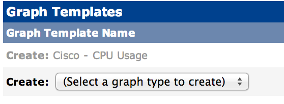
Once you have successfully created the host, you’ll be redirected to the details of that host and have the option to create graphs. Clicking on that link brings you to a page listing the Graph Templates that are associated with the device. Simply check the box next to the graphs that you want to create and click Create.

Within the next five minutes (the default polling interval), you should start seeing new data being graphed for the device you just created. Here is an example Hourly graph for a very low-usage switch port. The stair steps are due to the default polling cycle, which at five minutes is probably a bit too long by today’s standards. The green area is the inbound traffic, and the blue line represents the outbound. This graph template also includes the 95th percentile (not actually visible on the graph)--a very common way of billing network traffic, which is usually bursty in nature.

You can easily look at graphs for a specific host, but that’s not always the most useful way to see the data. Another feature of Cacti is called Graph Trees. Graph Trees allow you to create a folder-like structure for sorting and viewing your graphs. Want to look at the network throughput of all of your Raspberry Pis at once? No problem! Here we create a Switch heading in the Default Tree that only contains graphs we care about:

To view all our hard work, we move away from Console to the Graph view in Cacti. These two modes distinguish configuration from normal use and slightly change the interface. Don’t worry, though: it’s just clicking what looks like a tab at the top of the page to toggle back and forth.

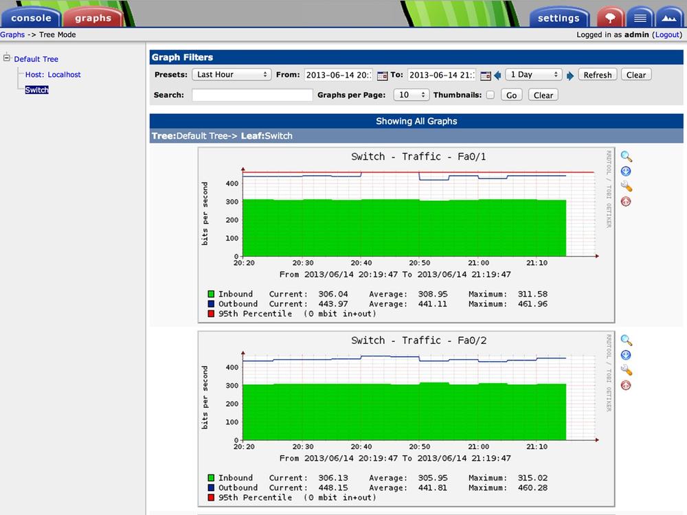
This is the Graphs view of Cacti, which contains the Graph Tree on the left, a quick filter across the top, and the resulting graphs in the main body. This is also where Cacti shows some of its age. While the page is mostly dynamic content, there is no AJAX in use, so the page refreshes via a meta tag, and you cannot directly interact with the graphs to change the time range you’re looking at.

If you’re paying close attention, you might have noticed that these graphs are for the Last Hour and are showing data from the Hourly RRA. If you want to see all the time periods for a specific graph, just click on it and you will be taken into the entire stored history of that data. This is very useful for identifying trends over time, which hopefully lets you plan for future growth.

Link Layer Discovery Protocol (LLDP) is one of the most under-utilized yet extremely useful networking protocols you may never have heard of. Ever unplug the wrong server from a switch because of out-of-date documentation or spaghetti wiring? Yeah, me either…but now you can know exactly which port a server is plugged into with confidence! You just need to enable LLDP on your switch and install lldpd.

It is important to note that there are other Link Layer protocols that have been implemented by multiple network equipment vendors over the years. LLDP was defined by IEEE 802.1AB to provide a vendor-neutral specification. This is an important step, as now cross-vendor devices could finally exchange information, and network engineers were pleased. Now it’s time to spread the information out to a broader audience.

While the inner working of LLDP is beyond the scope of this paper, the basics are quite simple. A device, be it a server, switch, router, or anything else, sends information about itself at regular intervals out of all connected network interfaces. This information typically includes the system name, name of the interface the data was sent on, and the system management IP address.

The receiving device then collects that data, adds what interface it saw that data coming from, and stores it for a specific amount of time. The data is only exchanged between devices directly connected over Ethernet, so you now can be certain which neighbor is really on a specific interface.

Capability Codes: R - Router, T - Trans Bridge,
                  S - Switch, H - Host, I - IGMP, r - Repeater
Device ID   Local Intrfce   Capability   Platform   Port ID
rpi-1       Fas 0/2         H            Linux      eth0
rpi-2       Fas 0/1         H            Linux      eth0

In this example from an old Cisco switch, we have two Linux hosts connected. So if I need to disconnect the eth0 interface from rpi-1, I know that it is plugged into the local port FastEthernet 0/2 of the switch. I can also tell that rpi-2 is not another switch, as the Capability column identifies it as H, which means it is a host.

There are a few implementations of LLDP for Linux: Open-LLDP, ladvd, and lldpd. I prefer lldpd for its simplicity of configuration, it’s ability to speak other proprietary discovery protocols like Cisco Discovery Protocol, and multiple output formats of the client utility.

Depending on what distribution you are running, lldpd might not be available as a package, but compilation and installation is standard. Once you have the package installed, there really isn’t much to the configuration. For example, when using the Rasbian package for installation, all you need to do is start the daemon to get up and running. Enabling CDP requires a slight modification to the configuration, as follows:

/etc/defaults/lldpd

# Start SNMP subagent and enable CDP
DAEMON_ARGS="-x -c"

Once you have lldpd installed and running, it only takes a few seconds for data to start coming in from your neighboring devices. The command to view the current LLDP information is lldpctl, and by default it prints out some very verbose information. In the following example, you can see that we are actually using CDP to communicate with a very old Cisco 2924 Switch:

-----------------------------------------------------------
LLDP neighbors:
-----------------------------------------------------------
Interface: eth0, via: CDPv2, RID: 4, Time: 8 days, 00:58:39
Chassis:
ChassisID: local switch.example.com
SysName: switch.example.com
SysDescr: cisco WS-C2924-XL
MgmtIP: 192.168.1.2
Capability: Bridge, on
Port:
PortID: ifname FastEthernet0/2
PortDescr: FastEthernet0/2
VLAN: 1, pvid: yes VLAN #1

So far all of this has been useful information for humans to parse, but that’s not really the scale I want to work at. lldpdctl helps us out by providing multiple output formats including key-value and XML. Here is the same example in key-value format for comparison:

$ lldpctl -f keyvalue
lldp.eth0.via=CDPv2
lldp.eth0.rid=4
lldp.eth0.age=8 days, 01:00:23
lldp.eth0.chassis.local=switch.example.com
lldp.eth0.chassis.name=switch.example.com
lldp.eth0.chassis.descr=cisco WS-C2924-XL
lldp.eth0.chassis.mgmt-ip=192.168.1.2
lldp.eth0.chassis.Bridge.enabled=on
lldp.eth0.port.ifname=FastEthernet0/2
lldp.eth0.port.descr=FastEthernet0/2
lldp.eth0.vlan.vlan-id=1
lldp.eth0.vlan.pvid=yes
lldp.eth0.vlan=VLAN #1

Now we have information on the server about how it’s connected to the rest of the world, in a parsable format, that with a little work we could pass to our configuration management software. One reason this becomes important is that it allows for automatic discovery of parent-child relationships between servers and the network equipment they’re attached to. With some simple wrapping—perhaps a custom fact if you are a Puppet user—you have the hostname of the switch you’re attached to (your parent). Now when you dynamically generate your monitoring configuration, you can pass along that you are connected to Switch.example.com.

A network can be a weird place, with ever-changing asymmetric paths moving bits from one place to another. Sometimes this leads to very different throughput performance between servers that appear to be otherwise identical. After running a few common utilities like traceroute—or perhaps curl on an HTTP service—you are still unable to replicate the problem.

Enter iperf, the network testing tool. Iperf is designed to measure the throughput between two points and runs as a client/server pair. It supports both UDP and TCP and can either test bidirectionally or unidirectionally from each endpoint in a single command. The power of iperf is how efficiently it is able to saturate a network connection. For TCP, it reports the overall throughput. For UDP, you can adjust the datagram size and the report includes throughput, packet loss, and jitter.

Installation is easy, as the package exists in most major Linux distributions and is supported for cross-platform compiling, and Windows binaries are available from third parties. To run iperf, you do need to have your firewall configured to allow connections between the two endpoints, with the default server port for TCP and UDP being 5001. You also need to have iperf running on both sides of the connection to test. Iperf can either run in Server or Client mode, one on each end of the connection, as in the following examples.

TCP Server Mode

$ iperf -s
-----------------------------------------------------------
Server listening on TCP port 5001
TCP window size: 85.3 KByte (default)
-----------------------------------------------------------
[ 4] local 192.168.1.101 port 5001 connected
     with 192.168.1.100 port 43697
[ ID] Interval Transfer Bandwidth
[ 4] 0.0-10.1 sec 114 MBytes 94.1 Mbits/sec

TCP Client Mode

$ iperf -c 192.168.1.101
-----------------------------------------------------------
Client connecting to 192.168.1.101, TCP port 5001
TCP window size: 22.9 KByte (default)
-----------------------------------------------------------
[ 3] local 192.168.1.100 port 43697 connected
     with 192.168.1.101 port 5001
[ ID] Interval Transfer Bandwidth
[ 3] 0.0-10.0 sec 114 MBytes 95.0 Mbits/sec

Performing an initial TCP test with iperf requires starting the server, then firing the client at it. In the above example, a Raspberry Pi is running as the server, with another system sending traffic to it. The end result is the complete throughput as measured from the client to the server. You can optionally measure both directions one at a time with the -r flag, or run both directions at the same time with the -d flag passed to the client. Which method to use depends on your expected workload, but in general you should get statistically similar results from the independent tests when each system is running on similar hardware.

UDP Server Mode

$ iperf -s -u
-----------------------------------------------------------
Server listening on UDP port 5001
Receiving 1470 byte datagrams
UDP buffer size: 160 KByte (default)
-----------------------------------------------------------
[ 3] local 192.168.1.101 port 5001 connected
     with 192.168.1.100 port 55272
[ ID] Interval      Transfer  Bandwidth  Jitter    Lost/Total
[ 3]  0.0-10.0 sec  114 MB    95.7 Mbps  0.158 ms     0/81482
[ 3]  0.0-10.0 sec  1 datagrams received out-of-order

UDP Client Mode

$ iperf -u -c 192.168.1.101
-----------------------------------------------------------
Client connecting to 192.168.1.101, UDP port 5001
Sending 1470 byte datagrams
UDP buffer size: 208 KByte (default)
-----------------------------------------------------------
[ 3] local 192.168.1.100 port 55272 connected
     with 192.168.1.101 port 5001
[ ID] Interval      Transfer  Bandwidth
[ 3]  0.0-10.0 sec  114 MB    95.8 Mbps
[ 3] Sent 81483 datagrams
[ 3] Server Report:
[ 3]  0.0-10.0 sec  114 MB    95.7 Mbps  0.158 ms     0/81482
[ 3]  0.0-10.0 sec  1 datagrams received out-of-order

Since UDP is stateless, it has no idea how far it can push the network like TCP does. So iperf has some sane defaults for sending UDP traffic, and by default targets 1Mbps of throughput. The previous examples worked around this by specifying our target bandwidth of 100M using the -b flag.

You may also notice that the UDP view on the client side also presents a Server Report. This is required since there are no guarantees with UDP—the client could happily send packets all day long to a server that was dropping them on the floor. Be mindful of this when comparing UDP results, as the client and server should agree.

MUltihost SSH Wrapper, or mussh, is truly an old utility that you can still find good use for today. At its core, mussh is just a shell script wrapper around SSH that allows you to execute the same command across multiple hosts either in sequence or parallel. The script has been filling a gap that until recently most CM tools have ignored: running one-off commands across your distributed systems.

We have configuration management, why would I possibly want to do something outside of that? While it is true that you should be enforcing system state with a bigger hammer, sometimes you only need to perform a task once, or infrequently.

Take for example NTP clock skew. I recently ran into an issue where I found that a service had a dramatically increased network queue time after a hardware upgrade. NTP configuration and service state were being enforced through CM, so I knew that it was running. I wanted to verify that all the system clocks were synchronized, and I didn’t want to manually ssh to each of them.

$ mussh -l pi -m 2 -h rpi-1 rpi-2 -c 'sudo ntpdate -u ntp.home'
pi@rpi-1: ntpdate: adjust time server ntp.home offset 0.0151 sec
pi@rpi-2: ntpdate: adjust time server ntp.home offset 0.0006 sec

Whoa, that’s a long command. So let’s break it down.

Sync NTP across multiple hosts concurrently

$ mussh 
  -l pi           # Set the ssh username
  -m 2            # Run on two hosts concurrently
  -h rpi-1 rpi-2  # Hostnames for the command
  -c ‘sudo ntpdate -u ntp.home’ # Sync ntp with this peer

The resulting output is in the format of hostname: output of the command, which is useful when you run commands that you expect a single line from. You can optionally pass the -b flag to have output buffered by mussh, otherwise the output from all systems will display interwoven with each other if you are expecting multiple lines of output per host.

We also make three assumptions in this example. The first is that you have key-based ssh authentication working between your computer and the list of hosts (you are using keys, right?). You also need to have ssh-agent running and working so you’re not prompted for your private key password for every host. Finally, this example assumes that the pi user is able to execute sudo on ntpdate without a password prompt, which works well for demos in a lab environment but is not a best practice for production.

Well, that’s all fine and dandy, but I don’t want to type all the server names in for every command! Luckily, mussh supports reading the hosts one line at a time out of a file with the -H option. So instead, grab them from whatever storage mechanism you have (flat-file, database, RESTful endpoint) and pipe them in!

$ grep "rpi-" servers.txt | mussh -l pi -H - -c 'uptime'
pi@rpi-1: 21:12:54 up 4 days, 23:18, 1 user, load average: 0.00
pi@rpi-2: 21:12:54 up 4 days, 23:18, 1 user, load average: 0.00

In this snippet, I’m searching through a text file for my Raspberry Pi “servers” and sending those through mussh. The secret is in the -H -, which tells mussh that the file to read from is stdin.

We still have a lot to learn from the past about where we can go in the future. The tools of our past live on and inspire innovation, daring us to replace them with the next generation. Some of the tools discussed here have successors that are still in infancy. Some of them are still in active development and could use an influx of motivated developers to push them to the next level. All of them have contributed to getting us where we are today and deserve—if nothing else—a tip of the hat.