
CHAPTER 2
RANKING WEB PAGES
One relatively new application of eigenvalues, eigenvectors, and a number of results and techniques in matrix computations and numerical analysis is on the problem of ranking web pages or documents. When we enter a query, say on Google's famous search engine, a long list of pages or web documents are returned as relevant, that is, documents that match or are related to the query in some way (in Section 3.5, we study how relevant documents are matched with a given query). However, the order in which these pages appear on our screen is far from arbitrary; they follow a determined order according to a certain degree of importance. For instance, if we enter the query “news”, and the first web pages on the list are cnn, msnbc, newsgoogle, foxnews, newsyahoo, and abcnews, that means that those news sources besides being related to the query, they are supposed to be more important than hundreds or thousands of other web pages related to news. But, how is this rank of importance determined? In particular, how is this done, taking into account the enormous size of the World Wide Web?
As we will see in this chapter, the mathematical modeling of the problem of ranking web pages leads to the problem of computing an eigenvector associated with the eigenvalue of largest magnitude. Obviously, this requires not only an efficient numerical method for this purpose, but also, given the special case of the huge matrix resulting from the modeling, it requires above all a feasible, simple, and hopefully fast numerical algorithm.
For reasons explained in detail later on, the numerical method of choice for this particular problem is the so–called power method, the simplest numerical method available for the computation of eigenvectors. On our way to determine conditions for the uniqueness of solution and for convergence, we will encounter and apply several important concepts and methods from linear algebra and matrix computations.

Figure 2.1 Modeling of Web page ranking
After studying the eigenvector approach, we will introduce relatively recent results on how to compute such a vector containing the ranks of web pages by using approaches other than the power method itself, and we will show that such alternative methods can be more computationally efficient. We stress again that the problem of ranking web pages is an elegant, illustrative, and obviously very useful real-world application of theory and techniques in linear algebra and matrix analysis.
2.1 THE POWER METHOD
Recall that given an n × n matrix A, a vector x ≠ 0 is called an eigenvector of A if
![]()
where λ is the corresponding eigenvalue. Similarly, a vector x ≠ 0 is called a left eigenvector of A if
![]()
Observe that a left eigenvector of A is in fact an eigenvector of AT, for the same eigenvalue λ.
In Section 1.10, we showed how to find eigenvalues and eigenvectors analytically, by solving the associated characteristic equation and a singular linear system, respectively. This is feasible as long as n is small. For large values of n, we have to use numerical methods. However, numerically approximating the eigenvalues and eigenvectors of a matrix A is not a very easy task; several sophisticated numerical methods have been developed for this task, the simplest of all of them is the so–called power method, which is however able to compute only the dominant eigenvector (the one associated with the eigenvalue of largest magnitude). For this reason, other methods are in general preferred over the power method, as most applications require the computation of more than just one of the eigenvalues or one of the eigenvectors. This had made the power method mostly just an illustrative introduction to the numerical computation of eigenvalues and eigenvectors.
Nevertheless, from the point of view of eigenvectors, the power method is now virtually the only method of choice for solving the problem of ranking web pages or documents, and search engines like Google make extensive use of this extremely simple but very effective numerical method, and it is in fact one of the main mathematical tools that Google and other search engines utilize. In the next sections, we explain in detail why this is so.
Let us start by describing how and why the power method works, and under what conditions. Assume that a matrix An×n has the following properties:
(a) it has a complete set of linearly independent eigenvectors v1,…,vn, and
(b) the corresponding eigenvalues satisfy
Observe the strict inequality in (2.1). We are interested in computing v1 – the dominant eigenvector, that is, the eigenvector associated with λ1. Assume now that we choose an arbitrary initial guess vector x0. Since the eigenvectors are linearly independent, then we can uniquely write
for some scalars c1,…,cn, with c1 ≠ 0.
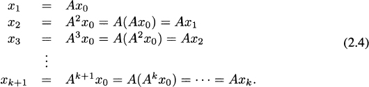
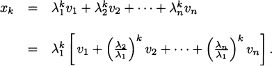
We can multiply both sides of (2.2) by A repeatedly and use the fact that Avi = λivi, for i = 1,… n, to obtain

Now recall that |λ1| > |λ2| ≥ ··· ≥ |λn|. Then, as k increases, the linear combination in Akx0 has more and more weight on the first term ![]() compared with any of the other terms. In other words, as k increases, the vector Akx0 moves toward the dominant eigenvector direction, and we expect that as k gets larger and larger, the vector Akx0 will converge to v1. That is exactly the main idea behind the power method.
compared with any of the other terms. In other words, as k increases, the vector Akx0 moves toward the dominant eigenvector direction, and we expect that as k gets larger and larger, the vector Akx0 will converge to v1. That is exactly the main idea behind the power method.
This means that it is not necessary to explicitly compute the powers of A, and instead just perform a matrix-vector multiplication Axk at each step.
The eigenvalue λ2 is called the subdominant eigenvalue and its corresponding eigenvector v2, the subdominant eigenvector. There is an important fact to observe in (2.3), especially in its last line: The farther |λ1| is from |λ2|, the faster the vector Akx0 will move toward the direction of the dominant eigenvector v1. That is, the speed of convergence depends on the distance between the dominant and subdominant eigenvalue (in magnitude), or more properly, on how small the ratio ![]() is.
is.
Now we collect the discussion above into the following
Theorem 2.1 Suppose the eigenvalues of a matrix An×n have the property
with corresponding linearly independent eigenvectors v1,…,vn. Then, for an arbitrary x0, the power iteration
converges to the dominant eigenvector v1, with rate of convergence
Consider the matrix

The eigenvalues are
![]()
Thus, the relationship |λ1| > |λ2| ≥ |λ3| ≥ |λ4| is satisfied, and the power iteration xk+1 = Axk will compute the dominant eigenvector
![]()
Here we show some of the iterates:

Computing the eigenvalue.
Although for the problem of ranking web pages we are not interested in finding the dominant eigenvalue (it will always be λ1 = 1), in general, one simple way to compute the eigenvalue λ associated with an already computed eigenvector v is derived from least squares. We begin by writing the equation Av = λv as
Equation (2.8) can be understood as a linear system with the (n × 1) coefficient matrix v. This system is overdetermined, and therefore (see Chapter 4), we look for its least squares solution, which is determined by solving the normal equations
![]()
from which we get
![]()
For instance, for the matrix A of Example 2.1, with v = [0 0 0 1]T, we have that Av = [0 0 0 −5]T, and
![]()
Some more details on this quotient are given in the Exercises section.
A different way to obtain the dominant eigenvalue is arrived at by first defining for a vector x = [x1 ··· xn]T the linear function
![]()
Now, on the last line of (2.3), we can absorb the constants c1,…,cn into the corresponding vectors v1,…,vn to obtain
![]()
where ![]() .
.
Now let
![]()
Since ![]() as k → ∞ and f is linear, we have that
as k → ∞ and f is linear, we have that
![]()
Thus, the ratio defined by μk approximates the dominant eigenvalue in an iterative process.
For the matrix of Example 2.1, we compute the dominant eigenvalue λ1 = −5 by following the ratio μ = f(xk+1)/f(xk), where we define f as f(x) = x4. These are some of the iterates

Going back to our original goal, we remark that there is more than one way to compute the (dominant) vector that contains the rank of all web pages. We cover here the method used by Google, not only because of its obvious practical importance and unquestionable success, but also because of the interesting mathematics behind it. First, we need to introduce three special types of matrices that will be encountered when developing the so–called PageRank algorithm.
2.2 STOCHASTIC, IRREDUCIBLE, AND PRIMITIVE MATRICES
The entire web will be represented as a directed graph, where each node on the graph is a web page. In turn, a particular matrix will be associated with this graph, so that such matrix will represent the web pages and their links to each other (see Figure 2.1). After some modification, the original matrix will be nonnegative, that is, a matrix with nonnegative entries, and each entry will lie in the interval [0, 1], with each row adding to one. It will be a stochastic matrix.
Definition 2.2 A matrix An×n is called (row) stochastic if it is nonnegative and the sum of the entries in each row is 1.
Note: In a similar way, we can define a column stochastic matrix as the one with the property that the sum of the entries in each column is 1. Observe that in any case, this means that all the entries of a stochastic matrix are numbers in the interval [0, 1].
Due to their special form, stochastic matrices have all their eigenvalues lying in the unit circle. In fact, we have the following theorem.
Theorem 2.3 If An×n is a stochastic matrix, then its eigenvalues have the property
![]()
and λ = 1 is always an eigenvalue of A.
Proof. Since the spectral radius of a matrix A never exceeds the norm of A (see Exercise 1.15), and since A is stochastic, then
where ![]() is the ∞ or 1-matrix norm, depending on whether A is row or column stochastic, respectively. On the other hand, let
is the ∞ or 1-matrix norm, depending on whether A is row or column stochastic, respectively. On the other hand, let ![]() be a vector of ones. Because A is stochastic, we either have Ae = e or eTA = eT(ATe = e) depending whether A is row or column stochastic respectively. That is, λ = 1 is always an eigenvalue of A. But this also means that ρ(A) ≥ 1, which combined with the inequality in (2.9) implies that ρ(A) = 1. Therefore, every eigenvalue of A must satisfy |λ| ≤ 1.
be a vector of ones. Because A is stochastic, we either have Ae = e or eTA = eT(ATe = e) depending whether A is row or column stochastic respectively. That is, λ = 1 is always an eigenvalue of A. But this also means that ρ(A) ≥ 1, which combined with the inequality in (2.9) implies that ρ(A) = 1. Therefore, every eigenvalue of A must satisfy |λ| ≤ 1.
The eigenvalues of the stochastic matrix
are (in order of magnitude):
![]()
This example shows that a stochastic matrix can have more than one eigenvalue of magnitude one.

The matrix A has eigenvalues λ1 = 1, λ2 = −1, λ3 = 0, λ4 = 0, so two of them have magnitude 1.
Definition 2.4 A matrix An×n is called reducible if there is a permutation matrix Pn×n and an integer 1 ≤ r ≤ n − 1 such that
where 0 is an (n − r) × r block matrix. If a matrix A is not reducible, then it is called irreducible.
Remark 2.5 Observe that equation (2.10) is a statement of similarity between the matrix A and a block upper triangular matrix.
From Definition 2.4, we can conclude two things:
- (a) A positive matrix (all its entries are positive) is irreducible.
- (b) If A is reducible, it must have at least (n − 1) zero entries.
However, a matrix with (n − 1) or more zero entries is not necessarily reducible, as in the case of the matrix of Example 2.3, which is irreducible.
It is of course not simple to conclude that a given matrix is irreducible or not by just looking at it, or by trying to find the permutation matrix P that would transform it into the canonical form (2.10). However, if we have a web or a graph associated with the matrix, it is much simpler to deduce the reducibility property of the matrix, at least for small n.
Definition 2.6 Given a matrix An×n, the graph Γ(A) of A is a directed graph with n nodes P1, P2,…,Pn such that
![]()
Note: Conversely, given a directed graph Γ(A), the associated matrix A will be called the link matrix, or adjacency matrix.
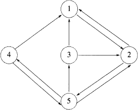
Figure 2.2 Web of Example 2.5.
Definition 2.7 A directed graph is called strongly connected if it there exists a path from each node to every other node.
This definition says that every node is reachable from any other node in a finite number of steps.
Consider the matrix of Example 2.3. The associated graph Γ(A) is shown in Figure 2.2. We observe that every node in the graph is reachable from any other given node. Thus, Γ(A) is strongly connected. The associated matrix A is irreducible.
The fact that the graph Γ(A) in Example 2.5 is strongly connected and the associated matrix A in Example 2.3 is irreducible is a consequence of a general result that can be stated as follows.
Theorem 2.8 A matrix An×n is irreducible ⇔ Γ(A) is strongly connected.
Proof. Assume that Γ(A) is not strongly connected. After a relabeling process, assume that S1 = {P1,…,Pr} is the set of all nodes that cannot be reached from node Pn. If we denote S2 = {Pr+1,…,Pn−1}, then no node in S1 can be reached from any node in S2 (Figure 2.3). Thus, if we denote with P the permutation matrix associated with the relabeling process, then we can write
![]()
where C is square of order r and 0 is an (n − r) × r block matrix. C represents S1 and E represents S2 ∪ {Pn}. This implies A is reducible.
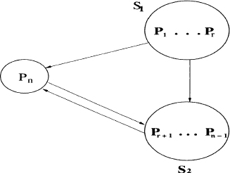
Figure 2.3 The graph Γ(A) in Theorem 2.8.
Conversely, assume A is reducible. Then, from Definition 2.4, there is a permutation matrix Pn×n such that
![]()
where 0 is a (n − r) × r block matrix, with 1 ≤ r ≤ n − 1. This means that the nodes P1,…,Pr in Γ(B) cannot be reached from any of the nodes Pr+1,…,Pn, and therefore, Γ(B) is not strongly connected. But, as noted before, because Γ(A) is the same as Γ(B) up to a renumbering of the nodes, (see Example 2.6), Γ(A) is also not strongly connected.
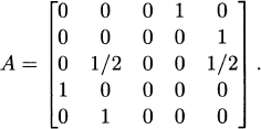
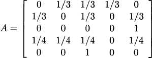
Consider the matrix

The associated graph Γ(A) is shown in Figure 2.4. We observe that the graph is not strongly connected. In particular, nodes 1 and 2 are not reachable from nodes 3 or 4. According to Theorem 2.8, this means the matrix A is reducible. In fact, we can transform A into the general reducible form (2.10) by permuting its rows and columns:
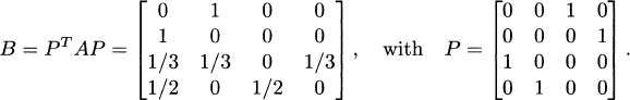

Figure 2.4 Web of Example 2.6
Note. Observe that the graph Γ(B) is the same as Γ(A) but with its nodes reordered according to the permutation assigned by P; that is:
![]()
Remark 2.9 Even though the two matrices in Examples 2.5 and 2.6 are stochastic, in general, reducible or irreducible matrices need not be stochastic.
When developing an algorithm to compute the rank of web pages, we will be interested in computing the dominant eigenvector of a link matrix. In general, for nonnegative matrices, there is an important theorem that provides conditions for the existence and uniqueness of such an eigenvector. This theorem is a generalization to nonnegative matrices of one originally proposed by Perron for positive matrices. The key property is that of irreducibility. Recall that ρ(A) denotes the spectral radius of A; that is,
![]()
Theorem 2.10 (Perron-Frobenius) Let An×n be a nonnegative irreducible matrix. Then,
- (a) ρ(A) is a positive eigenvalue of A.
- (b) There is a positive eigenvector v associated with ρ(A).
- (c) ρ(A) has algebraic and geometric multiplicity 1.
In general, a matrix may have a spectral radius that is not an eigenvalue itself. For instance we may have the eigenvalues σ(A) = {−4, −2, −1, 3}. In this case, ρ(A) = 4, but 4 is not an eigenvalue of A. Also, ρ(A) may be an eigenvalue but with algebraic multiplicity greater than one. For instance, we may have the case σ(A) = {2, 3, 4, 4}, where ρ(A) = 4 is an eigenvalue of algebraic multiplicity 2.
It is very important to stress that Theorem 2.10 guarantees that the vector space spanned by the dominant eigenvector is one-dimensional, which after normalization, it means that we will have a unique dominant eigenvector. For the purpose of ranking web pages, we will be looking for an eigenvector that is a probabilistic vector, that is, a vector with entries between 0 and 1, and with the sum of its components equal to one. That is, the 1-norm of the dominant eigenvector v = [v1 … vn]T is
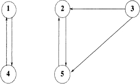
Figure 2.5 Web of Example 2.7.
![]()
Let us illustrate what may happen when irreducibility fails and the Perron–Frobenius theorem cannot be applied.
The following nonnegative matrix is reducible
The graph Γ(A) is shown in Figure 2.5. The eigenvalues of A are σ(A) = {1, 1, −1, −1, 0}. Thus, the spectral radius ρ(A) = 1 is an eigenvalue of A, with algebraic multiplicity 2. Furthermore, its associated dominant eigenvector is of the general form v = [a b 0 a b ]T. Thus, not only it is not positive, but the presence of two free variables a and b means that the eigenspace is two-dimensional. In fact, two linearly independent (normalized) eigenvectors can be chosen as ![]() and
and ![]() .
.
From Example 2.7, we learn that if the matrix is reducible (the corresponding graph is not strongly connected), we may have a problem of uniqueness of the dominant eigenvector when computing web pages rankings. For instance, which of the two vectors in such example should we pick as the right PageRank vector? Furhtermore, since they are linearly independent, any combination of them will also be in the same eigenspace.
Remark 2.11 If a web is considered as an indirected graph (links but no arrows), and it consists of k disconnected subgraphs, it can be proved that the corresponding dominant eigenspace has dimension at least k. See Exercise 2.25.
A general nonnegative matrix that is irreducible is already very special according to Theorem 2.10, especially because ρ(A) is an eigenvalue of algebraic and geometric multiplicity 1. But for the convergence of the power method, we will need the additional ingredient that ensures that the strict inequality in (2.5) is satisfied, that is, that the matrix in consideration should have only one eigenvalue of maximum magnitude.
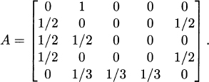
The matrix

is stochastic and irreducible, and therefore, ρ(A) has algebraic and geometric multiplicity one. However, it does not have a unique eigenvalue of largest magnitude. In fact, its eigenvalues are σ(A) = {1, −1, ±i}, all of them with magnitude 1. For this matrix, the strict inequality in (2.5) is not satisfied.
If we add the condition we need, then we get the following definition.
Definition 2.12 A nonnegative matrix An×n is called primitive if it is irreducible and has only one eigenvalue of maximum magnitude.
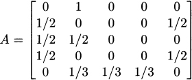
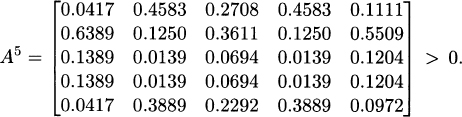
The matrix A of Example 2.3 is nonnegative and irreducible. In addition, its eigenvalues are λ1 = 1, λ2 = −0.9173, λ3,4 = −0.0413 ± 0.2986i, and λ5 = 0. Therefore, A is primitive as it has only λ1 = 1 as the dominant eigenvalue.
There is a useful characterization of primitive matrices that allows us to identify them without computing the eigenvalues.
Theorem 2.13 A nonnegative matrix An×n is primitive if and only if
Observe that according to this theorem, primitive matrices are just a generalization of positive matrices. In fact, a positive matrix is a primitive matrix with k = 1 in (2.11).
For the same matrix of Example 2.3, one can verify that A is primitive, with k = 5. In fact,
2.3 GOOGLE'S PAGERANK ALGORITHM
After covering Sections 2.1 and 2.2, we have the basic background to introduce a well–defined algorithm for ranking web pages. The fundamental numerical method to compute the dominant eigenvector is the power method, and the matrix under consideration will be modified to be stochastic. After a second modification, it will be not only irreducible, but it will be even primitive, fulfilling all the conditions for convergence to a unique eigenvector, the PageRank vector. It all starts with the original ideas of Google's founders Larry Page and Sergey Brin, and their article [11].
Before Google was available, entering a query online in search of information meant obtaining several screens of web pages or documents which happened to match the search text, but the order in which they were shown was not efficient. To locate an important document out of the long list, one had to scroll down and first read a long list of pages of dubious source that besides matching the text were not necessarily reliable or useful. The main reason behind Google's great success is that its PageRank algorithm is able to give very reliable rates of importance to all web pages in the world, so that after a query, it presents the user with a list of web pages or documents starting with the most important and typically most relevant ones. In this chapter, we review the mathematical concepts and tools used to develop the PageRank algorithm and we discuss how a direct application of such mathematical concepts as well as some practical manipulation of the algorithm itself have led to its success.
Because web pages are supposed to be listed in order of importance, the first question to answer was how to define the importance of a web page. The reasoning is that if a page is important (e.g., Google, Yahoo, top universities, etc.), then a great number of other web pages will have links to it. Thus, a way to define the importance of a page is by counting the number of inlinks to it. In this context, a link from page P1 to page P2 can be understood as page P1 “voting” for page P2. However, to avoid one page exerting too much influence by casting multiple votes, these votes should be scaled in some way. At the same time, votes from important pages should be ranked higher than those from ordinary ones. Altogether, this should result on each page having a rank of importance.
The central ideas in the PageRank algorithm can be summarized as:
(a) The rank of a page P is determined by adding the ranks of the pages that have outlinks pointing to P, weighted by the number of outlinks of each of those pages. This means for instance that if pages P1 and P2 point to page P, and P1 has 15 outlinks, while P2 has 100 outlinks, then the link from P1 will be given given more weight than P2. Each vote or link from P1 is worth 1/15, while each vote from P2 is only worth 1/100.
(b) In addition, links from important pages (revered authors, top-rank colleges, etc.) will have a higher weight than ordinary web pages.
If we denote the rank of a given page Pj with r(Pj), then part (a) can be expressed mathematically as

where Bpj is the set of all pages P pointing to Pj, and |P| denotes the number of outlinks from P. This obviously means that some initial ranks have to be assigned to all web pages (otherwise formula (2.12) is self-referencing), and the ultimate rank has to be determined as an iterative process.
Thus, if we consider n web pages, the rank of page Pj at step k is defined as
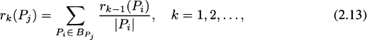
where i, j = 1,…,n and i ≠ j.
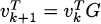
If we denote vk = [rk(P1) rk(P2) ··· rk(Pn)]T. Then, equation (2.13) can be expressed as

Thus, the equation ![]() is nothing else but the power method, in this case to compute the dominant (left) eigenvector of H associated with the eigenvalue λ = 1. The associated (dominant) eigenvector
is nothing else but the power method, in this case to compute the dominant (left) eigenvector of H associated with the eigenvalue λ = 1. The associated (dominant) eigenvector
is called the rank vector or PageRank vector.
Note. It is also possible to define the PageRank vector when the matrix H is column stochastic. See Exercise 2.63.

Figure 2.6 Web of Example 2.11.
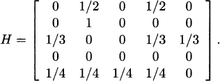
Consider the web of Figure 2.6 with four pages (or nodes). By observing how the pages are linked to each other, and following the definition in (2.14), we obtain the link matrix

Thus, the small web in Figure 2.6 consisting of four pages can be represented as a matrix H whose element hij can be defined as the probability of moving from node i to node j in one step (that is, in one mouse click).
In the matrix H of Example 2.11 we see that each row adds up to 1; in other words, H is a (row) stochastic matrix. Observe also that the third row has only one nonzero entry. This is because page 3 links only to one page; but this also implies that its vote for page 1 has the largest weight possible, a great benefit for page 1. The votes of the other pages are weighted so that all votes from one page have a total weight of one. In addition, H has a zero diagonal because the case of a page voting for itself is not considered. This is a good example of democracy.
Let us consider the web of Figure 2.7. The corresponding link matrix is given by
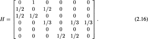
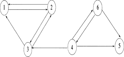
Figure 2.7 Web of Example 2.12.
The fact that page 5 does not have any outlinks is reflected in the matrix H having a corresponding row of zeros. This matrix is not stochastic. At the same time, H is reducible; in fact it can be written in the general reducible form (2.10), for a suitable permutation matrix P, and its graph is not strongly connected.
Example 2.12 is a simple illustration of what is to be expected in the real case of the World Wide Web: there will be several pages or documents with no outlinks (e.g., most PDF files), causing the corresponding link matrix to have a number of zero rows; in addition, because a given web page outlinks only to a few other pages, out of the several billions of pages available, the link matrix representing the entire World Wide Web will be very sparse and therefore, almost certainly reducible.
Here we discuss these two main issues, and how they can be resolved before one can proceed to apply power method to compute the pagerank vector v in (2.15).
(i) Making the matrix H stochastic.
As observed in Example 2.12, some of the rows in H may fail to add up to one because there is the possibility that some pages have no outlinks, and therefore, H will have some rows of zeros. Such a page or node is usually referred to as a dangling node. There is an easy solution to this problem: Just artificially add links by replacing the zero row with a nonzero vector. This is achieved by adding the matrix auT to H, where u is an arbitrary probabilistic vector (say, u = e/n, with e is a vector of ones), and a is a vector with entry i equal to 1, if page i is a dangling node; all other entries are zero.
More precisely, we define
This will modify only the zero rows, leaving the other rows untouched. Every zero row is effectively replaced by a probabilistic vector. This new matrix B is stochastic, and hence, the corresponding modified web has no dangling nodes.
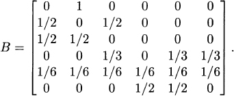
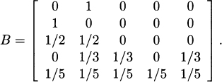
The matrix H of Example 2.12 has one row of zeros. By using (2.17), with u = e/6, we define
![]()
and e a vector of ones, to obtain

In the new web represented by B, page 5 now would link to all other pages and each of its votes is worth 1/6.
Remark 2.14 Observe that in Example 2.13, true democracy has been sacrificed because page 5 now has a vote for itself. However, in practice this does not represent a big concern. In general, due to the huge size of the web, each vote of a page that originally was a dangling node is actually worth almost nothing, e.g., 1/n, where n is in the order of billions. Thus, for the World Wide Web practical purposes, B is still very close to the original model represented by H and basically, the relationship between the ranks of the pages is not much affected.
Remark 2.15 Defining the matrix auT, with u = e/n may be overkill by completely filling up rows of zeros. Recall that u is an arbitrary probabilistic vector, so that e.g., in Example 2.13 we could define
![]()
so that the the fifth row of the matrix B in (2.19) equals this vector u and some sparsity is preserved. Later we will see that this type of choice for u gives other additional advantages.
(ii) Making the matrix B irreducible.
Remember from Section 2.2 that if a matrix is irreducible, then (after normalization), there is a unique dominant eigenvector. If this condition fails, then we face a problem of uniqueness. The issue of reducibility happens when for example a web page Pi contains only a link to page Pj, and in turn Pj contains only a link to Pi, then a surfer hitting any of these two pages is virtually trapped bouncing between Pi and Pj forever. More generally, in the language of graphs, and as noted in Theorem 2.8, reducibility happens when the web is not strongly connected; that is, not every node or page is reachable from any given arbitrary node.
To ensure irreducibility, Google forces every page to be reachable from every other page. This is very reasonable from the practical point of view, because a surfer can eventually jump to any page entering a URL on the command line, no matter from which page.
The strategy is to add a perturbation matrix to B, and let
where α ∈ (0 1). The matrix E can be defined as
where again, e is a vector of ones, and the arbitrary probabilistic vector u is called the personalization vector, a vector that has a great role in the success of Google's search engine. The stochastic irreducible matrix G is what we can call the “Google matrix”.
The two choices of perturbation matrices in (2.21) are quite different. Every entry in the matrix E = eeT/n is given by Eij = 1/n, so that every page will have its rank equally modified. This is the choice that Google used in its first years, but for several reasons that we explain below, now the second choice is being used. Also observe that the first choice of E is just a particular case of the second one, with u = e/n.
The matrix B of Example 2.13 is stochastic but reducible, because it can be expressed in the general form of (2.10) with r = 3. By taking the first choice in (2.21) we perturb B to make it irreducible, and for α = 0.8 we define according to (2.20)
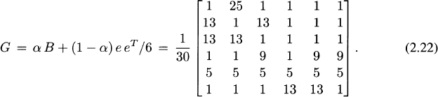
All the entries are now positive, and that obviously makes G irreducible. In terms of the web it means every page is now reachable from any other page; that is, the associated graph is strongly connected.
The two major technical problems with the original matrix H have been solved above by making some modifications to such matrix so that it is stochastic and irreducible. But as observed in Example 2.14, even more has been obtained because the general Google matrix G in (2.20) has all its entries strictly positive. This also makes it primitive! Therefore, now we also know that λ = 1 is the only eigenvalue of G of largest modulus, thus satisfying the condition (2.5) for the convergence of the power method.
In fact, if we apply the power method to (2.22), it will uniquely converge to its normalized dominant (left) eigenvector (the PageRank vector):

Figure 2.8 A primitive matrix satisfies all conditions needed
That is, this vector v satisfies
![]()
Suppose now that a query is entered, and the pages (or documents) 1, 2, 4, and 5 are returned as relevant; that is, they match the query. Then, these four pages will be shown to the user, but they will be arranged in the order given by the corresponding entries in the PageRank vector; that is,

With the properties of the matrix G, convergence of the power method to a unique PageRank vector is now guaranteed, and one can proceed to compute such a vector (see Figure 2.8). However, there are a couple more issues we want to discuss.
First, besides a page being important in terms of how many inlinks it receives from other pages, it would be a great advantage to be able to manipulate some of the ranks so that really important pages are ensured to get a well–deserved high rank; at the same time the ranks of pages of financially generous businesses could also be pushed up, making sure their products will be listed first. These considerations have been implemented in PageRank and have put Google at the top of search engines. And second, nothing has been said about the speed of convergence, whether there could be some ways to improve the rate of convergence of the power method, and whether the sparsity of the original matrix H can still be exploited, although from (2.22) we can see that it has been lost.
It is remarkable to learn that all these issues can be solved by manipulating the entries of the personalization vector u in (2.21), by giving an appropriate value to α in (2.20,) and by rewriting the power method to avoid using the matrix G explicitly.
2.3.1 The personalization vector
Recall that we have modified the original link matrix H to make it stochastic and irreducible, and that the final matrix G in (2.20) we have obtained is even primitive, so that all conditions are given for uniqueness and convergence when applying the power method. Now we consider the second and more general choice in (2.21); that is, we take
where e is a vector of ones, and the vector u is in general an arbitrary probabilistic vector: its entries lie between 0 and 1, and they add up to 1.
It is this vector u that allows us to manipulate the PageRank values up or down according to several considerations. Thus, home pages of revered authors, top schools, or financially important businesses can be assigned higher ranks by appropriately fixing the entries of u. At the same time for reasons like spamming attempts or artificially trying to manipulate their own ranks, other pages can be pushed down to lower ranks.
To show how effective this approach can be, we will consider again the matrix B (2.19) from Example 2.13.
After modification of the original link matrix H, we have the matrix
To make this matrix reducible, we perturb as in (2.20), with α = 0.8. Suppose now that we want to promote page 5 to a much higher rank. Then, we can define the probabilistic personalization vector
![]()
Now by taking the second choice in (2.21), we get

When we apply the power method to this matrix G, we get the PageRank vector
Thus, assuming again that after entering a querry, pages 1,2 4, and 5 are the relevant ones, now they will be shown to the user in the following order:
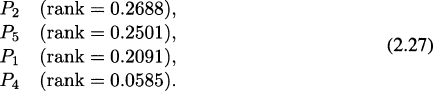
It is obvious in Example 2.15 that with that choice of a personalization vector, we force the rank of page 5 up from v5 = 0.0900 to v5 = 0.2501, a huge increase indeed (the new rank is almost three times the original one). This has moved page five to appear second in the list, with a rank very close to that of page 2. The ranks of all pages other than 5 have decreased.
This is how ranks of a few web pages can be accommodated so that they appear in a somehow prescribed order of importance. Nevertheless, this must be done carefully and applied to modify only a very few number of pages; otherwise, this notion of importance would be in clear conflict with that of relevance, that is, which pages actually are closer to the query.
2.3.2 Speed of convergence and sparsity
To ensure uniqueness of the PageRank vector associated with the dominant eigenvalue λ = 1, the original link matrix H representing the web has been modified according to (2.17) to obtain a stochastic matrix B, and then B itself has been modified according to (2.20) to obtain the stochastic irreducible (and in fact, primitive) matrix G. Also recall that with this matrix G, the condition (2.5) is satisfied and the convergence of power method is guaranteed.
One very important thing to note is that although the Google matrix G still has all of its eigenvalues lying inside the unit circle, they are in general different from those of B. What is surprising is that instead of causing any trouble, this has a positive effect on the algorithm itself and it can be effectively exploited.
Theorem 2.16 Denote the spectra of B and G with
Then,
where α is as in (2.20).
Proof. Let ![]() so that
so that ![]() , for i = 1,…,n. Since B is row stochastic, we have Bq = q. Now let X be a matrix so that
, for i = 1,…,n. Since B is row stochastic, we have Bq = q. Now let X be a matrix so that
![]()
is orthogonal (see orthonormal extensions in Section 1.4.7). Then,
![]()
On the other hand, for u a probabilistic vector and e a vector of ones,

Then,

From the first similarity transformation QTBQ, we see that the eigenvalues of C are {μ2,…,μn}, and from the second one QTGQ, we conclude that indeed the eigenvalues of G satisfy λk = αμk, for k = 2, 3,…,n.
Consider the matrices B and G of Example 2.15, where we set α = 0.8. Their eigenvalues are
![]()
Thus, we see that indeed λk = αμk, for k = 2,…, 6.
Remark 2.17 The proof of Theorem 2.16 can also be done by constructing a nonsingular (and not necessarily orthogonal) matrix U = [q X], where q is an eigenvector of U. See Exercise 2.46.
As discussed in Section 2.1, the speed of convergence of the power method depends on the separation between the dominant eigenvalue and the subdominant eigenvalue. One problem with B was that the subdominant eigenvalue μ2 may be too close or even equal to the dominant eigenvalue μ1 = 1, because B is not primitive. The usefulness of Theorem 2.16 is that when we have the matrix G, since λ2 = αμ2 and α lies in the interval (0, 1), we can choose α away from 1, to increase the separation between λ1 = 1 and λ2 and, hence, speed up the convergence of the PageRank algorithm. It has been reported that Google uses a value of α between 0.8 and 0.85.
Observe that the choice of α affects how much the matrix B is modified in (2.20), and therefore it also affects the importance of the personalization vector u in (2.21). In other words, the parameter α and the vector u give Google the freedom and power to manipulate and modify page ranks, according to several considerations. Every time a surfer enters a query, there is the confidence that the pages returned are sorted in the right order of importance. At the same time, we just saw that the choice of α also gives control on the speed of convergence of the algorithm. Taking α far from 1 will cause the algorithm to converge faster and gives a larger weight to the perturbation matrix E = euT and therefore to the personalization vector u. However, α cannot be taken too far from 1, because that will take the matrix G too far from B, and that would not be an accurate model of the original web.
As for sparsity, the original matrix H is very sparse because each page has only very few links to other pages (and remember there are billions of those pages). This sparsity is only barely affected by B. However, the matrix G in (2.20) is positive and has no zero entries anymore, so that in principle sparsity is completely lost. Fortunately this does not represent any problem in practice. Remember we need to apply the power method to find the dominant left eigenvector of G with eigenvalue λ = 1; that is, we are interested in the iteration
![]()
From (2.17) and (2.20), and using the fact that ![]() , we have the following two cases, depending on whether u = e/n, or u is an arbitrary probabilistic vector.
, we have the following two cases, depending on whether u = e/n, or u is an arbitrary probabilistic vector.
If u = e/n, then
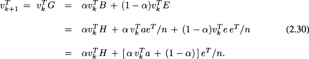
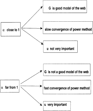
Figure 2.9 How α affects web page ranking.
If u is arbitrary, then

Thus, in both cases, the only matrix-vector multiplication is ![]() , so that sparsity is preserved, something that can be fully exploited in practical terms. Also, the only vector-vector multiplication is
, so that sparsity is preserved, something that can be fully exploited in practical terms. Also, the only vector-vector multiplication is ![]() , where a is a very sparse vector. Furthermore, the calculations above also show that the matrices B and E do not need to be formed explicitly. All this is possible because of the simplicity of the power iteration. In general this would not be possible for more sophisticated numerical methods, and that makes the power method just about the only feasible algorithm for computing the dominant eigenvector (the PageRank vector) of the very large Google matrix G.
, where a is a very sparse vector. Furthermore, the calculations above also show that the matrices B and E do not need to be formed explicitly. All this is possible because of the simplicity of the power iteration. In general this would not be possible for more sophisticated numerical methods, and that makes the power method just about the only feasible algorithm for computing the dominant eigenvector (the PageRank vector) of the very large Google matrix G.
Computing the vector a. Recall that the n-dimensional vector a contains the information about which pages are dangling nodes, or which is the same, which are the zero rows of H. See (2.18). For small n, the entries of a could found by hand; e.g., in Example 2.12, the vector a is simply a = [0 0 0 0 1 0]T.

Figure 2.10 Matrix H for Example 2.17
In general, for a large sparse matrix H of order n, we can obtain a by using the following MATLAB commands:

This tells MATLAB to initially create a sparse vector a of zeros and then change the entry to 1 if the corresponding row sum of H is zero.
Datasets representing a given web are typically stored as an n × 3 array. By instance, a web (or graph) generated after the query “California” can be stored as

The first two columns represent the pages numbers, and the third is the weight of the link. In particular, page 1 has 17 outlinks, page 2 links only to page 483, page 3 has exactly three outlinks: to pages 484, 533, and 583, and so on. There are n = 9,664 pages in total in this example.
Then, using MATLAB we can convert this dataset into an n × n link matrix H and visualize its sparsity pattern, where each blue dot represents a nonzero entry. See Figure 2.10.
- MATLAB commands: spconvert(H), spy(H)
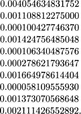
Power method (2.30) with α = 0.83 converges to the PageRank vector in 72 iterations, with an error 3.6502 × 10⁻⁹. These are the ranks of pages P1 to P10:
Remark 2.18 If in Example 2.17 we use α= 0.95, then to achieve an error of about10−9, we need 261 iterations (more than three times the number of iterations needed with α = 0.83). This illustrates how α determines the speed of convergence of the power method.
2.3.3 Power method and reordering
As discussed before, the larger the gap between |λ1| and |λ2|, the faster the power method will converge. Some theoretical results indicate that some reorderings speed up the convergence of numerical algorithms for the solution of linear systems. The question is whether some similar matrix reorderings can increase the separation between the dominant and the subdominant eigenvalue. For the particular case in mind, since λ1 = 1, we would like to see whether some matrix reordering can take |λ2| farther from 1.
Extensive testing shows that by performing row and column permutations so as to bring most nonzero elements of the original matrix H say to the upper left comer, causes the gap between |λ1| and |λ2| to increase, and therefore, power method converges in fewer iterations.
- MATLAB commands: Colperm(H), fliplr(H)
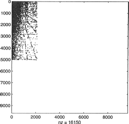
Figure 2.11 Reordered California matrix H.
When the power method with reordering is applied to the California dataset of Example 2.17 (n = 9,664), convergence is achieved in only 21 iterations, clearly better than the 72 iterations needed without permutation. As for clock time, including reordering, it is about 15% faster. Similarly, for a dataset Stanford, with n = 281,903, power iteration without reordering needs 66 iterations to converge, whereas with reordering only 19 iterations are needed. The total time for convergence, including reordering, is about 66% shorter than the power method without reordering.
In Figure 2.11, we show the reordered matrix H of Example 2.17. Compare this with Figure 2.10. If we want to visualize the original Stanford matrix we would mostly see a solid blue square, even though it is a sparse matrix. The reordered Stanford matrix is shown in Figure 2.12.
2.4 ALTERNATIVES TO THE POWER METHOD
The size of the link or adjacency matrix associated with the graph representing the entire World Wide Web has made the very simple power method and its modifications just about the only feasible method to compute the dominant eigenvector (the PageRank vector) of G. More sophisticated methods for computing eigenvectors turn out to be too expensive to implement. In recent years, however, researchers have been looking for alternative and hopefully faster methods to compute such PageRank vector. A first approach transforms the eigenvector problem into the problem of solving a linear system of equations. A second approach aims at reducing the size of the eigenvector problem by an appropriate blocking of the matrix G. We investigate these two different approaches and how they can be combined to build up more efficient algorithms.

Figure 2.12 Reordered Stanford matrix H.
2.4.1 Linear system formulation
The motivation behind expressing the problem of ranking web pages as a linear system is the existence of a long list of well–studied methods that can be used to solve such systems. The central idea is to obtain a coefficient matrix that is very sparse; otherwise, the huge size of the matrix would make any linear system solver by far much slower than the power method itself.
We start by observing that for 0 < α < 1, the matrix I−αHT is nonsingular. Indeed, the sum of each column of the matrix αHT is strictly less than one and therefore ![]() . Then, according to Exercise 1.22, the matrix I − αHT must be nonsingular.
. Then, according to Exercise 1.22, the matrix I − αHT must be nonsingular.
That the eigenvector problem to compute the PageRank vector is equivalent to the problem of solving a linear system is expressed in the following theorem.
Theorem 2.19 Let G = αB + (1 − α)euT, where B is as in (2.17) and 0 < α < 1. Then,

Proof. By substituting G = α(H + auT) + (1 − α)euT into vT = vTG and using the fact that vTe = 1, we have that
![]()
which can be written as vT(I − αH − αauT) = (1 − α)uT, or equivalently
The coefficient matrix in the linear system (2.33) is a rank-1 modification of the matrix I − αHT, and therefore, we can apply the Sherman–Morrison formula (see Exercise 2.67) to get
![]()
where M = I − αHT. Thus, if x is the solution of Mx = u, then the solution of (2.33) can be computed explicitly as
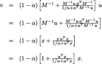
Thus, the PageRank vector v is just a multiple of x and we can use the constant ![]()
![]() to normalize v so that
to normalize v so that ![]() .
.
Let us go back to the matrix H of Example 2.12. It was found later in Example 2.14 that the corresponding PageRank vector, that is the vector v that satisfies vT = vTG was
![]()
If instead we solve the system (I − αHT)x = u, with u = e/n and e a vector of ones as usual, we get
![]()
Then, after normalizing ![]() we get exactly the same PageRank vector v.
we get exactly the same PageRank vector v.
Remark 2.20 The rescaling of the vector x to obtain v in Theorem 2.19 is not essential because the vector x itself already has the correct order of the web pages according to their ranks. Also since in principle we only need to solve the linear system (I − αHT)x = u, the rank-1 matrix auT(which was introduced to take care of the dangling nodes) does not play a direct role.
Through Theorem 2.19, the eigenvector problem vT = vTG has effectively been transformed into solving a linear system whose coefficient matrix I − αHT is just about as sparse as the original matrix H. This gives us the opportunity to apply a variety of available numerical methods and algorithms for sparse linear systems and to look for efficient ways and strategies to solve such systems as a better alternative to finding a dominant eigenvector with the power method.
2.4.1.1 Reordering by dangling nodes The sparsity of the coefficient matrix in the linear system (2.32) is the main ingredient in the linear system formulation of the web page ranking problem. However, due to the enormous size of the web, we should look for additional ways to reduce the size of the problem or the computation time. One simple but very effective way to do this is by reordering the original matrix H so that zero rows (the ones that represent the dangling nodes) are moved to the bottom part of the matrix. This will allow us to reduce the size of the problem considerably. The more dangling nodes the web has, the more we can reduce the size of the problem through this approach.
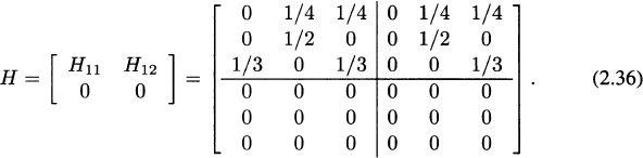
By performing such reordering, the matrix H can be written as
where H11 is a square matrix that represents the links from nondangling nodes to nondangling nodes and H12 represents the links from nondangling nodes to dangling nodes. In this case, we have
![]()
and therefore the system (I − αHT) x = u is
![]()
which can be written as

Thus, we have an algorithm to compute the PageRank vector v:
- Reorder H by dangling nodes.
- Solve the system
 .
. - Compute
 .
. - Normalize
 .
.
Through this algorithm, the computation of the PageRank vector requires the solution of one sparse linear system ![]() , which is much smaller than the original one in (2.32), thus effectively reducing the size of the problem. The computational cost of steps 1,3, and 4 of the algorithm is very small compared to that involved in the solution of the linear system itself.
, which is much smaller than the original one in (2.32), thus effectively reducing the size of the problem. The computational cost of steps 1,3, and 4 of the algorithm is very small compared to that involved in the solution of the linear system itself.
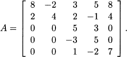
Consider the matrix

When we reorder by dangling nodes, we get
Let u = [0.1 0.2 0.1 | 0.4 0 0.2]T = [u1 u2]T, and α = 0.8. Following (2.35), the solution of the system ![]() is
is
![]()
and ![]() gives
gives
![]()
Then, by normalizing the vector x = [x1 x2]T, we get
![]()
This vector v is the pagerank vector of the matrix G in Theorem 2.19, with H given in (2.36). In fact, that matrix G is given by
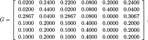
Its dominant eigenvector is
![]()
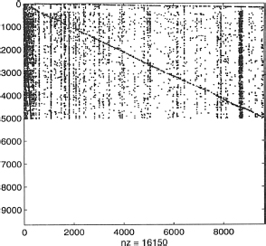
Figure 2.13 Reordered matrix H for Example 2.20.
which, after normalization in the 1-norm, gives again the vector v found above.
Note that this vector x is different than the vector x = [x1 x2]T above, but they are multiples of each other.
Let us consider the matrix Hn×n of Example 2.17, where n = 9,664, and let u = e/n, where e is a vector of ones. Instead of using the power method, we can solve the linear system (2.32), or first reorder such matrix H by dangling nodes (see Figure 2.13) and then apply (2.35). For the given example, since the number of dangling nodes of the original matrix H is r = 4637, the sparse block matrix H11 is square of order n − r = 5027. Once the matrix is reordered, the algorithm runs about 55% faster than the one without reordering.
2.4.2 Iterative aggregation/disaggregation (IAD)
Another attempt to outperform the power method in the computation of the PageRank vector comes from the theory of Markov chains. A Markov chain is a stochastic process describing a chain of events. Suppose we have a set of states S = {s1,…,sn} and a process starts at one of these states and moves successively from one state to another. If the chain is currently at state si then it moves to state sj in one step with probability pij, a probability that depends only on the current state. Thus, it is clear that such a chain can be represented by a stochastic matrix Gn×n (called the transition matrix), with entries pij.
If the transition matrix is irreducible, the corresponding Markov chain is also called irreducible. In such a case, a probabilistic vector v is called is called a stationary distribution of the Markov chain if
![]()
This means that the PageRank vector (the dominant left eigenvector of G we are interested in) is also the stationary distribution of the Markov chain represented by the matrix G.
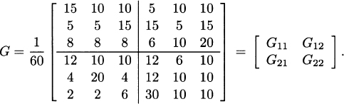
The main idea behind the IAD approach to compute the PageRank vector v is to block or partition the irreducible stochastic matrix G so that the size of the problem is reduced to about the size of one of the diagonal blocks. Thus, let
It can be shown that (I − G11) is nonsingular. Then, define

where
S is called the stochastic complement of G22 in G, and it can be shown to be irreducible and stochastic if so is G. Then we have
![]()
Thus,
![]()
because U is nonsingular. The last equation reduces to
which in particular implies that
![]()
That is, v2 is a stationary distribution of S. If u2 is the unique stationary distribution of S with ![]() , then we must have
, then we must have
![]()
for some scalar c. It remains to find an expression for v1.
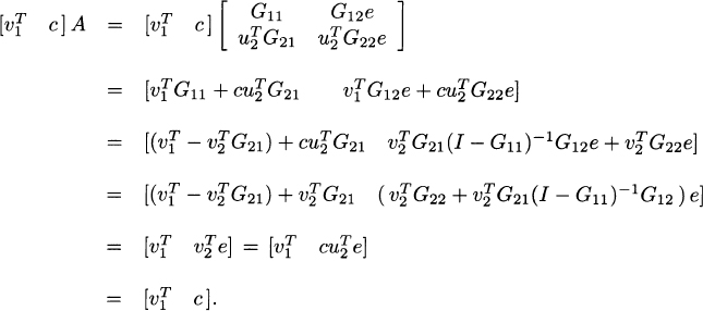
Associated with G there is the so–called aggregated matrix, defined as
where e represents vectors of ones of appropriate size and u2 is as defined above. First we want to find the stationary distribution of A.
Observe that from (2.40), we can get ![]() , which means
, which means
![]()
At the same time, the equation ![]() implies that
implies that
![]()
We then have
We can now summarize the discussion above into the following theorem.
Theorem 2.21 (Exact aggregation/disaggregation)
If u2 is the stationary distribution of S = G22 + G21(I − G11)−1G12 and ![]() is the stationary distribution of
is the stationary distribution of ![]() , then the stationary distribution of
, then the stationary distribution of
![]()
is given by ![]() .
.
The computation of the matrices S and A and their corresponding stationary distributions is the aggregation step, while forming the vector v = [v1 cu2]T is considered to be the disaggregation step.
Consider the stochastic irreducible matrix
The stationary distribution of S = G22 + G21(I − G11)−1G12, with ![]() is
is

The stationary distribution of ![]() , where the vector e is e = [1 1 1]T, is given by
, where the vector e is e = [1 1 1]T, is given by

Therefore, the stationary distribution of G, with ![]() is
is

That is, it satisfies vT = vTG, with ![]() .
.
Through Theorem 2.21, the problem of computing the stationary distribution of G has been split into finding stationary distributions of two smaller matrices. Observe however that forming the matrix S and computing its stationary distribution u2 would be very expensive and not efficient in practice. The idea is to avoid such computation and use instead an approximation.
More precisely, we define the approximate aggregation matrix:
where ![]() is an arbitrary probabilistic vector that plays the role of the exact stationary distribution u2.
is an arbitrary probabilistic vector that plays the role of the exact stationary distribution u2.
Such approximation is reasonable because the matrix ![]() differs from the original matrix A only in the last row, while typically, G11 is in the order of billions of rows for the PageRank problem. It can be shown that
differs from the original matrix A only in the last row, while typically, G11 is in the order of billions of rows for the PageRank problem. It can be shown that ![]() is irreducible and stochastic if so is G; thus, we are guaranteed that
is irreducible and stochastic if so is G; thus, we are guaranteed that ![]() has a unique stationary distribution.
has a unique stationary distribution.
In general, this approach does not give a very good approximation to the stat ionary distribution of the original matrix G, and to improve accuracy, a power method step is applied. More precisely:
To compute an approximate stationary distribution ![]() of G, we apply the following approximate aggregation/disaggregation algorithm:
of G, we apply the following approximate aggregation/disaggregation algorithm:
- Select an arbitrary probabilistic vector
 .
. - Compute the stationary distribution
 of
of  .
. - Let
 .
.
Typically, we will have ![]() so that the actual algorithm to be implemented consists of repeated applications of the algorithm above. That is, we start with an arbitrary
so that the actual algorithm to be implemented consists of repeated applications of the algorithm above. That is, we start with an arbitrary ![]() , compute the stationary distribution of
, compute the stationary distribution of ![]() and form
and form ![]() . For the next iteration,
. For the next iteration, ![]() is taken as the second block of the current vector
is taken as the second block of the current vector ![]() . Then we repeat the process until convergence.
. Then we repeat the process until convergence.
That is, we have the following iterative aggregation/disaggregation(IAD) algorithm:
- Give an arbitrary probabilistic vector and a tolerance

- For k = 1, 2,…
- Find the stationary distribution of
- Set

- Let
- If
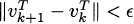 , stop. Otherwise,
 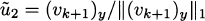 .
.
- Find the stationary distribution
Here, (vk+1)y denotes the second block of the vector vk+1.
2.4.2.1 IAD and power method Upon examining the IAD algorithm above, we see that we need to compute ![]() , the stationary distribution of
, the stationary distribution of ![]() . This vector satisfies
. This vector satisfies

Thus, we can use the power method to solve for it. However, we are faced again with the same problem: the matrices G11, G12, G21, and G22 that make up ![]() are full matrices and applying the power method directly would not be efficient.
are full matrices and applying the power method directly would not be efficient.
The question is whether we can still apply a strategy similar to (2.30) and (2.31) so that we are able to exploit the sparsity of the original link matrix H.
We start by writing the matrix ![]() as (Exercise 2.80)
as (Exercise 2.80)
![]()
so that we drop G22. We can simplify further by setting ![]() , and thus
, and thus ![]() becomes
becomes
![]()
From (2.43), we have

To explicitly get some sparsity, first we write G in terms of H as before:
![]()
Then we block the matrices H, auT and euT according to the blocking of G:
for some matrices A, B, C, D, E, F, J, and K.
Now we see that
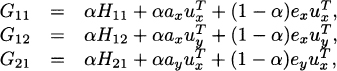
where the subindices x and y denote blocking of the vectors a, u, and e according to the blocking of G. Thus, e.g., ax denotes the first block of entries of the vector a with size corresponding to the size of G11.
Now we can use the sparsity of H11, H12, and H21 to make computations simpler and faster. The equations in (2.44) can now be written as

For the iterative process of the power method within IAD, we give as usual an arbitrary initial guess ![]() and iterate according to (2.46) for the next approximation
and iterate according to (2.46) for the next approximation ![]() until certain tolerance is reached.
until certain tolerance is reached.
Exploiting dangling nodes. Although not obvious in (2.46), it is possible to exploit not only the sparsity of the matrices H11, H12, and H21 but also some reorderings applied to H. Fy instance, if H is reordered by dangling nodes, bringing all the zero rows to the bottom of the matrix, then the matrix H21, which is used in ![]() is a matrix of zeros. Also, by definition of the vector a (see (2.18)), we will have all the entries of ax to be zeros. All this reduces power method computation in (2.46) to
is a matrix of zeros. Also, by definition of the vector a (see (2.18)), we will have all the entries of ax to be zeros. All this reduces power method computation in (2.46) to

Some other reorderings can even transform H12 into a zero matrix reducing computations even more.
2.4.3 IAD and linear systems
The two alternatives to the original power method we have presented above are a linear systems approach and IAD, both offering some clear advantages over the original algorithm. We want to illustrate how both approaches can be combined to provide an improved algorithm for the computation of the pagerank vector.
Recall that within the IAD algorithm we need to compute the stationary distribution of the approximate aggregation matrix ![]() . This has been done by applying the power method to
. This has been done by applying the power method to
![]()
Now we want to rewrite this equation so that we can arrive at the solution by solving some linear system. We have
After multiplication, we get
![]()
which can be written as
Observe that the first equation in (2.49) is a linear system of the order of G11 and the second one is just a scalar equation. However, such a system with coefficient matrix I − G11 cannot be solved because the right–hand side contains ![]() , which is unknown.
, which is unknown.
Thus, the idea is initially to fix an arbitrary ![]() so that the system
so that the system ![]() can be solved, and once w1 is computed, we can adjust
can be solved, and once w1 is computed, we can adjust ![]() using the second equation in (2.49). This approach is reasonable because, as remarked before, for the application in mind, G11 has billions of rows while
using the second equation in (2.49). This approach is reasonable because, as remarked before, for the application in mind, G11 has billions of rows while ![]() is just a scalar.
is just a scalar.
More precisely, to compute the stationary distribution ![]() of
of ![]() , we apply the following algorithm.
, we apply the following algorithm.
- Give an initial guess
 and a tolerance .
 - Repeat until
 :
:
- Solve
 .
. - Adjust
 .
.
- Solve
Typically it takes just a couple of steps to reach a given tolerance ![]() so that this computation is relatively fast in terms of number of iterations. However, the matrices G11, G12, and G21 are full matrices so that computations at each step are in general very expensive. Thus, similarly to what it was done when studying IAD with the power method, we go back to the original matrix H to get some sparsity.
so that this computation is relatively fast in terms of number of iterations. However, the matrices G11, G12, and G21 are full matrices so that computations at each step are in general very expensive. Thus, similarly to what it was done when studying IAD with the power method, we go back to the original matrix H to get some sparsity.
From equation (2.45), we can look at G11 in more depth to get
The last term, ![]() can disturb the sparsity of I − G11, but we will use the fact that
can disturb the sparsity of I − G11, but we will use the fact that ![]() to simplify. We know this to be true because
to simplify. We know this to be true because
![]()
We also know that
![]()
which can be used to keep the system sparse. With this knowledge, our linear system, ![]() , becomes
, becomes
Thus, to compute w1, we solve the linear system
Dangling nodes. Similarly as before, some reorderings of the matrix H can mean a reduction of the computational cost in the solution of the linear system. Thus, e.g., assume that H has been reordered by dangling nodes, i.e, the zero rows have been moved to the bottom part. In such a case, we have
![]()
so that H21 is a matrix of zeros. Then we have the following theorem.
Theorem 2.22 Let the matrix H be reordered by dangling nodes. Then, the system (2.52) reduces to
Proof. Due to the reordering by dangling nodes, the vector ax is a vector of zeros and the vector ay is a vector of ones, of the same size as ey, so that ay = ey. Since ![]() is a probabilistic vector, we also have
is a probabilistic vector, we also have ![]() . Then, we can simplify equation (2.52) to
. Then, we can simplify equation (2.52) to

Simply by reordering the matrix, in this case by dangling nodes, a computation that could have been time consuming has now been effectively simplified.
Following a similar reasoning, one can prove that the computation of the scalar ![]() can also be reduced in the case of a link matrix H that has been reordered by dangling nodes. More precisely, since
can also be reduced in the case of a link matrix H that has been reordered by dangling nodes. More precisely, since
![]()
and ![]() , calculations similar to those in Theorem 2.22 reveal that we can compute
, calculations similar to those in Theorem 2.22 reveal that we can compute ![]() as
as

Thus, our algorithm that combines the ideas from IAD and linear systems, with the original link matrix H arranged by dangling nodes, can be expressed in a simplified form as
Finally, we remark again that some particular reorderings of H can additionally give H12 = 0, simplifying computations even more.
2.5 FINAL REMARKS AND FURTHER READING
The problem of ranking web pages is a real-world application of some concepts and techniques from matrix algebra and numerical analysis. We have presented the minimum theoretical background necessary to build well-defined algorithms, and we have presented some examples with matrices of relatively small size. The starting and most basic algorithm is the power method, but recent studies have shown that a linear system approach and aggregation methods can also be applied and combined to achieve faster convergence. In all cases, permutations or reordering of the link matrices are important to develop more efficient algorithms.
The fundamental background needed is a set of results on nonnegative matrices. The book by Berman and Plemmons [4] offers a sound analysis of the most important properties of stochastic, irreducible, primitive, as well as M-matrices. Langville and Meyer [44] have studied the PageRank algorithm in detail and have reported their findings in several works including [44], [45], and [50]. Ipsen and Kirkland [39] provide with details on the convergence of an IAD algorithm developed by Langville and Meyer. A detailed report on the linear system approach for finding the PageRank vector can also be found in the work by del Corso et al. [16]. Osborne et al. [53] first combine power method with matrix reorderings and then combine the IAD approach with both, power method and linear systems, to obtain algorithms with fast convergence to the PageRank vector. As for other approaches toward improving the computation of webpage ranking, the work by Berkhin [3] proposes a bookmark coloring algorithm, with a predefined threshold value that induces sparsity and faster speed of convergence. In Andersen and Peres [2], an algorithm for PageRank computation is improved and further applied to develop Page Rank-Nibble, a very efficient algorithm for local graph partitioning.
Research in this area of matrix computations applied to search engines is very active, and new and novel results are expected in the near future. More and more efficients algorithms are needed as the size of the World Wide Web increases by the millions every day. Thus, for realistic situations, the size of the matrices involved make the use of supercomputers and parallelism a must.
EXERCISES
Do the eigenvalues of A satisfy the condition (2.5)? If so, apply the power method to find the dominant eigenvector. What is the rate of convergence?
2.2 Find a matrix An×n and give an initial guess ![]() so that the power method xk+1 = Ax1 does not converge.
so that the power method xk+1 = Ax1 does not converge.
2.3 Rewrite the last equation in (2.3) as

where we assume again that |λ1| > |λ2| ≥ ··· ≥ |λn|. Define the sequence ![]()
![]() , k = 0, 1, 2,…, and show that
, k = 0, 1, 2,…, and show that
![]()
for some constant C and for any vector norm ![]() . Thus, uk → c1v1, as k → ∞.
. Thus, uk → c1v1, as k → ∞.
2.4 Assume a matrix An×n is nonsingular. Explain how you would modify the power method algorithm to compute an eigenvector associated with the smallest eigenvalue. What conditions must the eigenvalues of A satisfy?
2.5 Let u and v be nonorthogonal vectors. The quantity
is called the generalized Rayleigh quotient. If u is an eigenvector of A, then the Rayleigh quotient gives the corresponding eigenvalue. Now consider a nonzero vector v and define the so–called residual r(μ) = Av − μv. Show that ![]() is minimized when
is minimized when
This μ is commonly known as the Rayleigh quotient.
2.6 Let x be a unit eigenvector of An×n with associated eigenvalue λ. Consider the Rayleigh quotient μ in (2.57), with ![]() . Show that
. Show that
![]()
where ![]() .
.
2.7 Let v be an eigenvector of a matrix A, with corresponding simple eigenvalue λ. Consider the iteration
![]()
with ![]() , for all k, and assume that vk → v as k → ∞. Show that
, for all k, and assume that vk → v as k → ∞. Show that
![]()
for some constant C.
Hint. Use Exercise 2.6 and observe that the iteration above is the power method applied to (A − μk+1I)−1.
2.8 Consider the power iteration xk+1 = Axk, and suppose that for a given positive integer k, we have xk−2 = v1 + α2v2, where v1 and v2 are the dominant and subdominant eigenvectors of An×n, respectively. For i = 1,…,n, define the entries of vectors b, c, and d respectively, by
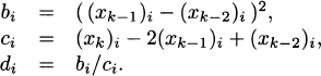
Show that v1 = xk−2 − d.
2.9 Show that a matrix An×n is stochastic if and only if
(a) Ax ≥ 0, for all vector x ≥ 0, and
(b) Ae = e, where e is a vector of ones.
2.10 Show that a matrix An×n is stochastic if and only if the vector w = uTA is a probabilistic vector, for every probabilistic vector u.
2.11 Show that the convex combination of two stochastic matrices is a stochastic matrix. That is, if A and B are stochastic, then the matrix
![]()
is also stochastic.
2.12 Show that if P is a stochastic matrix, then the matrix Pn is also stochastic for all integers n > 0.
2.13 Let Qn×n be an orthogonal matrix. Show that the matrix A defined by ![]() is column and row stochastic.
is column and row stochastic.
2.14 True or False? Every stochastic matrix A is nonsingular.
2.15 Let An×n be an arbitrary nonsingular nonnegative matrix, and let ![]() . Show that there exists a diagonal matrix D such that
. Show that there exists a diagonal matrix D such that
![]()
is stochastic.
2.16 Let An×n be a stochastic matrix and λ ≠ 1 an eigenvalue of A. Show that if v is a left eigenvector of A, then it is also a left eigenvector of the matrix B = (aij − cj), where ![]() .
.
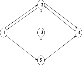
Figure 2.14 Graph of Exercise 2.22
2.17 Let An×n be a nonnegative matrix. Show that there exists a path of length k in Γ(A) from a node Pi to a node Pj if and only if (Ak)ij ≠ 0.
Hint. Use induction, starting with k = 2.
2.18 An alternative way of defining the spectral radius of a square matrix A is
Use this definition to prove the following: If A and B are nonnegative matrices, then
![]()
2.19 Let An×n be a nonnegative matrix. Show that
Hint: Construct a nonnegative matrix B that satisfies A ≥ B and whose row sums are all equal to ![]() .
.
2.20 Let An×n be a nonnegative matrix and ![]() a positive vector. Show that if Ax > rx for some scalar r > 0, then ρ(A) > r.
a positive vector. Show that if Ax > rx for some scalar r > 0, then ρ(A) > r.
2.21 Let An×n be a nonnegative matrix. Show that ρ(A) is a positive eigenvalue of A, and that there is a positive eigenvector associated with it.
2.22 Is the link matrix associated with the graph in Figure 2.14 irreducible?
2.23 Show that the matrix
is reducible by finding a permutation matrix P so that
![]()
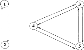
Figure 2.15 Graph of Exercise 2.28
for some matrices B, C, and D. Also draw the graphs Γ(A) and Γ(B).
2.24 Show that if A and B are nonnegative matrices and A is irreducible, then A + B is irreducible.
2.25 Show that if an undirected graph modeling a web consists of k disconnected subgraphs, then the dimension of the dominant eigenspace(the one spanned by the dominant eigenvector) is at least k.
2.26 Let B be a stochastic positive matrix. Show that any eigenvector v in the dominant eigenspace has either all positive or all negative entries.
2.27 Let B be a stochastic positive matrix. Without using the Perron–Frobenius Theorem 2.10, show that the dominant eigenspace has dimension one.
2.28 Consider the graph of Figure 2.15. Find the corresponding link matrix and the dimension of the dominant eigenspace.
2.29 Let An×n be a positive column stochastic matrix, and let S be the subspace of ![]() consisting of vectors v such that
consisting of vectors v such that ![]() . Show that S is invariant under A, that is, AS ⊂ S.
. Show that S is invariant under A, that is, AS ⊂ S.
2.30 Find a nonnegative matrix An×n, with at least one but not all entries equal zero, so that ρ(A) is a zero eigenvalue with algebraic multiplicity greater than one.
2.31 Is the matrix  irreducible?
2.32 Let A be a reducible matrix; that is, ![]() , for some permutation matrix P. Show that solving a system Ax = b can be reduced to solving the systems
, for some permutation matrix P. Show that solving a system Ax = b can be reduced to solving the systems
![]()
where ![]() , so that
, so that ![]() .
.
2.33 True or False? An irreducible matrix may have a row of zeros.
2.34 True or False? An irreducible matrix has at least one nonzero off-diagonal element in each row and column.
2.35 True or False? If a matrix A is reducible, then Ak is reducible for each k ≥ 2.
2.36 Consider the matrix

Verify that its spectral radius ρ(A) is an eigenvalue of algebraic and geometric multiplicity 1, yet the matrix A is reducible. Does this contradict Theorem 2.10?
2.37 Suppose that all row sums of a nonnegative matrix An×n are equal to a constant k. Show that ρ(A) = k.
2.38 Let An×n be a nonnegative matrix with row sums less than or equal to 1 (with at least one row sum strictly less than 1). Show that ρ(A) ≤ 1.
2.39 Find a stochastic irreducible matrix A that does not have a unique eigenvalue of largest magnitude.
2.40 Verify and apply the Perron–Frobenius theorem to the matrix

2.41 Let An×n be a primitive stochastic matrix. Show that the rows of the matrix
![]()
are all identical.
Hint: First show that every row of S is a left eigenvector of A with eigenvalue λ = 1.
2.42 Consider the matrix
What is ![]() ?
?
2.43 Show that if A and B are nonnegative matrices and A is primitive, then A + B is primitive.
2.44 True or False? The product of two primitive matrices is also a primitive matrix.
2.45 Let An×n be an irreducible stochastic matrix. Show that rank (I − A) = n − 1.
2.46 Give a slightly different proof of Theorem 2.16 by constructing a nonsingular matrix U = [q X], where q is an eigenvector of U.
2.47 Let Bn×n be a reducible matrix. Show that B is similar to a block upper triangular matrix. More precisely, show that there exists a permutation matrix P such that

where each Akk is irreducible or a zero scalar.
2.48 Let An×n be an irreducible and weakly diagonal dominant matrix. Show that all its diagonal entries are nonzero.
2.49 The following matrix H is neither stochastic nor irreducible. Follow the equations (2.17) and (2.20) with α = 0.8, u = e/5 and e a vector of ones to form a stochastic and irreducible matrix G.
2.50 The following matrix is stochastic but reducible. Apply equation (2.20) with α = 0.8, u = e/5, where e is a vector of ones, to make it irreducible, and then apply the power method to find the PageRank vector, that is, the dominant eigenvector v with ![]() .
.
What is the resulting order of the corresponding web pages in terms of importance?
2.51 Make the matrix B of Exercise 2.50 irreducible, with α = 0.8, but now using the personalization vector
![]()
What is the new order of importance of the web pages?
2.52 Given a stochastic matrix H representing a web, how would you quickly find a rough estimate of the order of the corresponding web pages in terms of importance?
2.53 Let Gn×n = αB + (1 − α)euT, where u = e/n and e is a vector of ones, and let ![]() . Show that
. Show that
![]()
and that μ is an eigenvalue of I + μeuT.
2.54 Find the eigenvalues of the matrices B and G = αB + (1 − α)euT, where

α = 0.8, u = [0.3 0.1 0.2 0.4 0]T, e is a vector of ones, and verify Theorem 2.16.
2.55 Consider the matrix

Let e be a vector of ones and u = e/5. Solve the system (I − αHT)x = u with α = 0.85 and then normalize ![]() . Verify the statement in Theorem 2.19 that this vector v is the PageRank vector of the matrix G = αB + (1 − α)euT, where B is as in (2.17).
. Verify the statement in Theorem 2.19 that this vector v is the PageRank vector of the matrix G = αB + (1 − α)euT, where B is as in (2.17).
2.56 Give a different proof of Theorem 2.19 by first proving that
![]()
and by observing that solving vT = vTG is equivalent to solving xT(I − G) = 0, where the PageRank vector v satisfies ![]() .
.
2.57 Show that the system (I − αHT)x = u in (2.32) has a unique solution.
2.58 We say a square matrix A is an M-matrix if and only if there exists a nonnegative matrix B and a real number k with ρ(B) ≤ k such that A = kI − B. Show that the matrix I − αH is an M-matrix, where H is the usual link matrix and 0 < α < 1.
2.59 Let the matrix ![]() be stochastic and irreducible. Show that the corresponding approximate aggregation matrix
be stochastic and irreducible. Show that the corresponding approximate aggregation matrix
![]()
is also stochastic and irreducible.
2.60 Let Gn×n be an irreducible stochastic matrix. Show that I − G is a singular M-matrix.
2.61 Let An×n be a singular irreducible M-matrix. First show that rank(A) = n − 1 and then show that there exists a positive vector x such that Ax = 0.
2.62 Let An×n be a matrix whose off-diagonal entries are nonpositive. Show that A is an M-matrix if and only if ![]() is a nonsingular M-matrix for all
is a nonsingular M-matrix for all ![]() .
.
2.63 Show that if the link matrix H is column stochastic, then the PageRank vector is ![]() , with
, with
![]()
where G = α(H + u aT) + (1 − α)ueT, e is a vector of ones, u is an arbitrary probabilistic vector, and 0 < α < 1. How do you define the entries of H?
2.64 Let u = e/7, where ![]() is a vector of ones. Reorder by dangling nodes the following matrix:
is a vector of ones. Reorder by dangling nodes the following matrix:

so that it takes the block form
![]()
Then solve the equations (2.35) to find the vector x that solves (I − αHT)x = u. Finally, normalize ![]() . Verify that this vector is the PageRank vector of the matrix G as given in Theorem 2.19.
. Verify that this vector is the PageRank vector of the matrix G as given in Theorem 2.19.
2.65 Consider the original matrix H of Example 2.19. Compute the PageRank vector by directly applying (2.32), that is, without reordering by dangling nodes, and compare your answer with the one in the Example.
2.66 Suppose the link matrix H is column stochastic. Show that
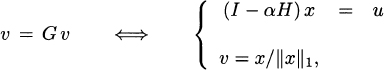
where G is as in Exercise 2.63.
2.67 Let An×n be nonsingular, and let ![]() be two vectors such that 1 + yTA−1x ≠ 0. Show that A + xyT is nonsingular and that
be two vectors such that 1 + yTA−1x ≠ 0. Show that A + xyT is nonsingular and that
![]()
This is known as the Sherman–Morrison formula.
Hint: First show that ![]() , for any two nonzero vectors u, v such that 1 + vTu ≠ 0.
, for any two nonzero vectors u, v such that 1 + vTu ≠ 0.
2.68 Suppose the link matrix H is column stochastic so that after reordering by dangling nodes, it can be expressed as
![]()
Show that the problem of solving the system (I − αH)x = u can be reduced in size in a similar way to (2.35).
2.69 Let u = e/7, where ![]() is a vector of ones. Reorder the following column stochastic matrix by dangling nodes
is a vector of ones. Reorder the following column stochastic matrix by dangling nodes
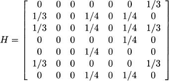
so that it takes the block form
![]()
Then solve the equations you found in Exercise 2.68 to find the vector x that solves (I − αH)x = u. Finally, normalize ![]() . Verify that this vector is the PageRank vector of the corresponding matrix G.
. Verify that this vector is the PageRank vector of the corresponding matrix G.
2.70 For the matrix G in Exercise 2.77, let S be the stochastic complement of G22. Find the unique stationary distribution u2 of S such that ![]() .
.
2.71 Consider the matrix G in Exercise 2.77. Find the corresponding aggregated matrix A and its probabilistic stationary distribution, and then find the stationary distribution v of G with ![]() .
.
2.72 Let ![]() be a row stochastic irreducible matrix with G11 a square block of order k. Let as usual ei(i = 1,…,n) represent the i–th canonical vector. Show that
be a row stochastic irreducible matrix with G11 a square block of order k. Let as usual ei(i = 1,…,n) represent the i–th canonical vector. Show that
![]()
where 1 ≤ i, j ≤ n − k.
2.73 Let G be a column stochastic irreducible matrix written as
Let S be defined as S = G22 + G21(I − G11)−1G12. If u2 satisfies Su2 = u2 and v2 is the unique dominant eigenvector of S with ![]() , that is, v2 = cu2, for some scalar c, show that the dominant eigenvector of G is given by v = [v1 v2]T, where
, that is, v2 = cu2, for some scalar c, show that the dominant eigenvector of G is given by v = [v1 v2]T, where
![]()
for some matrix A (this is the corresponding aggregated matrix).
2.74 Let G be a column stochastic irreducible matrix written as in (2.59). Show that the equations (2.49) are now of the form

![]()
be an irreducible stochastic matrix. Show that the matrix I − G can be factored as I − G = LDU, where L, D, and U are given in (2.38).
2.76 Show that the stationary distribution v of the matrix G in the previous exercise is given by
![]()
where as usual u2 is the unique stationary distribution of the stochastic complement S of G22, v2 = cu2, L is given in (2.38), and x is an arbitrary vector of appropriate size.
2.77 Consider the stochastic irreducible matrix

Compute the factorization
![]()
where L, D, U are given in (2.38).
2.78 Suppose that in the approximate aggregation disaggregation algorithm, the vector ![]() coincides with the unique stationary distribution of S; that is,
coincides with the unique stationary distribution of S; that is, ![]() . Show that the stationary distribution of G is exactly
. Show that the stationary distribution of G is exactly ![]() .
.
2.79 Let ![]() . Show that for an arbitrary vector x of appropriate size,
. Show that for an arbitrary vector x of appropriate size,
![]()
2.80 Show that the aggregated matrix (2.41) can be written as
![]()
2.81 Prove formula (2.55).
2.82 Show that the vector ![]() used in the definition of the approximate aggregated matrix
used in the definition of the approximate aggregated matrix ![]() can be computed as
can be computed as
![]()