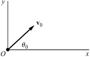
A small body falls downward with an initial velocity v0 from a height h near the surface of the earth, as in Figure 4.1.1. For low velocities (less than approximately 24 m/s), the effect of air resistance may be approximated by a frictional force proportional to the velocity. Find the displacement and velocity of the body, and determine the terminal velocity. Plot the speed as a function of time for several initial velocities.
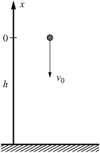
Let the x-axis be directed upward, as in Figure 4.1.1. The net force on the object is
where m is the mass, g is the magnitude of the acceleration due to gravity, and v is the velocity. The positive constant b depends on the size and shape of the object and on the viscosity of the air. From Newton’s second law, the equation of motion is
with x(0) = h and v(0) = v0. We can rewrite Equation 4.1.2, a second-order equation, as two first-order equations:
(For further discussion of falling bodies, see [Sym71]; for more information on the effects of retarding forces on the motion of projectiles, refer to [TM04].)
In[1]:= ClearAll ["Global'*"]
DSolve solves Equations 4.1.3 and 4.1.4 with the initial conditions x(0) = h and v(0) = v0:
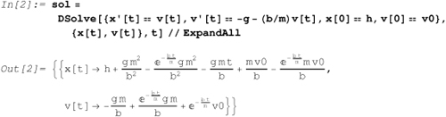
The solution for the displacement x(t) and velocity v(t) is given as a list of rules.
To determine the terminal velocity, let bt/m >> 1 in the rule for v(t):
The terminal velocity vt is –gm/b.
Let us determine the velocity as a function of time in a system of units where time, displacement, and, therefore, velocity are in units of m/b, gm2/b2, and gm/b, respectively:
We now plot the speed as a function of time for three illustrative initial velocities:
In[5]:= Plot[
         Evaluate[{Abs[v[t]] /. v0 → − 3, Abs[v[t]] /. v0 → − 0.6,
           Abs[v[t]] /. v0 → 0, 1}], {t, 0, 3.5}, PlotRange → All,
         Frame → True, FrameLabel → {"t (m/b)","speed (gm/b)"},
         PlotStyle → {{Red}, {}, {Blue}, {Dashing[{0.02}]}},
         Prolog → {Text["v0 = 0", {0.95, 0.3}], Text["|v0|}|vt|", {2.8, 0.55}],
           Text["|v0|>|vt|", {1.5, 2.05}], Text["terminal speed,|vt|",
            {0.9, 1.2}], Line[{{0.95, 0.79}, {2.2, 0.6}}]}]
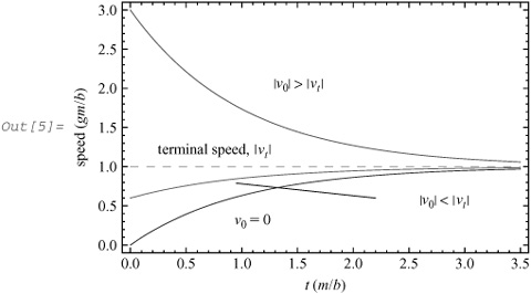
The bottom two curves indicate that the speed of the body increases, as expected, and eventually approaches the terminal speed during its descent. The top curve shows that if the initial speed exceeds the terminal speed, the falling object actually slows down and its speed approaches the terminal speed from above. (Note that although the velocity of the falling body is negative, its speed is positive.)
In[6]:= ClearAll [sol, v]
A baseball of mass m leaves the bat with a speed v0 at an angle θ0 from the horizontal. The effect of air resistance may be approximated by a drag force FD that depends on the square of the speed—that is,
FD = –mkvv
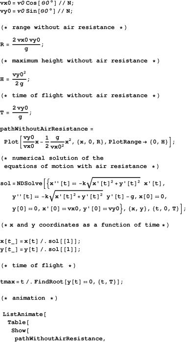
where v and v are the speed and velocity of the ball, respectively, and the drag factor k is equal to 5.2 × 10⁻³ m–1. Define a function that generates an animation of the motion of the baseball. The function should have v0 and θ0 as arguments, and the animation should show the paths of the baseball with and without air resistance. Evaluate the function for v0 = 45 m/s and θ0 = 60°.
The equations of motion for the baseball are


where the x and y directions are the horizontal and vertical directions, respectively, as in Figure 4.2.1, and g is the magnitude of the acceleration due to gravity.
If air resistance is negligible (i.e., k = 0), these equations can be solved analytically. The path of the baseball is given by the equation
where the initial position is chosen as the origin, and the initial x and y components of the velocity are
vx0 = v0 cos θ0
vy0 = v0 sin θ0
The maximum altitude occurs at
the range is
and the time of flight is
A realistic model for the flight of the baseball must include air resistance. Unfortunately, the equations of motion, Equations 4.2.1 and 4.2.2, can no longer be solved analytically; numerical methods must be employed. (For more information on the physics of baseball, consult [Ada95] and [Bra85].)
What follows is a function that generates an animation of the motion of the baseball. Comments giving the details about the function are embedded in the body of the function in the form (* comment *). These comments are ignored by the Mathematica kernel. The function takes two arguments: The first is the numerical value of the initial speed in SI units, and the second is that of the initial elevation angle in degrees. The initial speed is limited to 80 m/s because higher speeds are unlikely for baseballs, and the initial angle of elevation is restricted to the range 30° to 85° in order to accommodate the sizes of most monitor screens.
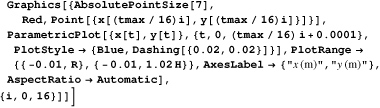
Let us generate the animation of the motion of the baseball with v0 = 45m/s and θ0 = 60°:
In[3]:= projectile [45, 60]
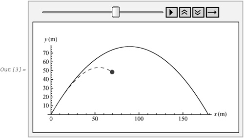
The solid line represents the path of the baseball without air resistance; the dashed line traces that with air resistance. To animate, click the Play button—that is, the one with the right pointer.
Solve the equations of motion numerically and plot the phase diagrams of the plane, the damped, and the damped, driven pendulums. For the damped, driven pendulum, also determine the Poincaré section and generate an animation of the pendulum.
Consider a particle of mass m that is constrained by a rigid and massless rod to move in a vertical circle of radius L, as in Figure 4.3.1. The equation of motion is
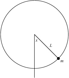
where x is the angle that the rod makes with the vertical,
and g is the magnitude of the acceleration due to gravity. We can rewrite Equation 4.3.1, a second-order equation, as two first-order equations:
If the unit of time t is taken to be t0 = 1/ω0, Equation 4.3.4 assumes the form
where x is in radians and v is in radians/t0.
We now include damping that is proportional to the velocity. Equation 4.3.5 becomes
where a is a parameter measuring the strength of the damping.
With a sinusoidal driving force, Equation 4.3.6 becomes
where F and ω are the amplitude and frequency of the driving force, respectively.
The motion of the pendulum depends on the parameters a, F, and ω as well as on the initial conditions for x and v. Whether the motion is periodic or chaotic is determined solely by the parameters a, F, and ω. (For introductions to chaotic dynamics, consult [BG96] and [TM04]; for more advanced discussions, refer to [Moo87], [Ras90], and [Hil00].)
In this section, we solve the equations of motion and plot the phase diagrams of the plane, the damped, and the damped, driven pendulums. For the damped, driven pendulum, we also determine the Poincaré section and generate an animation of the pendulum.
In[1]:= ClearAll ["Global' *"]
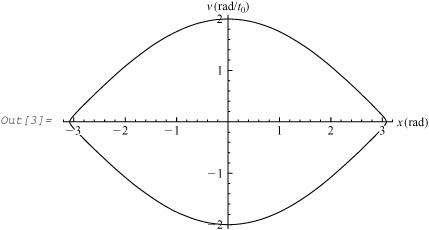
As an example, we choose the initial conditions x = 0 and v = 2 – d, where d is a small number. (What would happen if the initial conditions are such that x = 0 and v ≥ 2? See Problem 5 in Section 4.5.) NDSolve solves Equations 4.3.3 and 4.3.5 together with the initial conditions:
In[2]:= points1 = NDSolve [{x' [t] == v [t], v'[t] == - Sin [x[t]],
            x[0] == 0, v[0] == 2 − 0.001}, {x, v}, {t, 0, 19.5}];
With the solution points1, we can plot the phase diagram:
In[3]:= ParametricPlot[Evaluate[{x[t], v[t]} /. points1],
         {t, 0, 19.5}, AxesLabel → {"x (rad)", "v (rad/t0)"}]
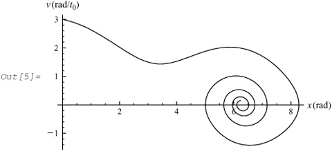
For an example, choose the initial conditions x = 0 and v = 3 and let a = 0.2. NDSolve solves Equations 4.3.3 and 4.3.6 together with the initial conditions:
In[4]:= points2 = NDSolve[{x'[t] == v[t], v'[t] == - Sin[x[t]] − 0.2 v[t],
            x[0] == 0, v[0] == 3}, {x, v}, {t, 0, 30}];
Let us plot the phase diagram:
In[5]:= ParametricPlot[Evaluate[{x[t], v[t]} /. points2],
         {t, 0, 30}, PlotRange → All, AxesLabel → {"x (rad)", "v (rad/t0)"}]
As an example, let a = 0.2, F = 0.52, and ω = 0.694:
In[6]:= {a, F, ω} = {0.2, 0.52, 0.694};
Also, choose the initial conditions x = 0.8 and v = 0.8.
For t in the range 0 to cycles(2π/ω), NDSolve solves Equations 4.3.3 and 4.3.7 together with the initial conditions:
In[7]:= cycles = 50;
         sol3 = NDSolve[{x'[t] == v[t],
              v'[t] == - Sin[x[t]] - a v[t] + F Cos[ω t], x[0] == 0.8, v[0] == 0.8},
             {x, v}, {t, 0, cycles(2 π/ω)}, MaxSteps → 20 000];
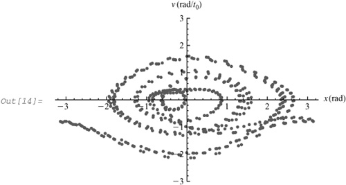
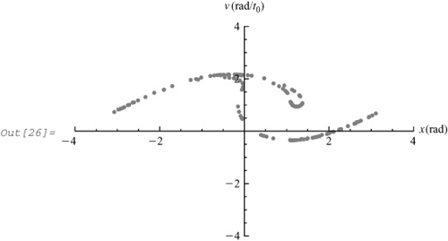
Mathematically, the angle x can take on values from –∞ to +∞; physically, x can only vary from –π to +π. In the following, the phase diagram is constructed with all the points translated back to the interval –π to +π and with the lines connecting adjacent points omitted for clarity:
In[9]:= reduce[x_] := Mod[x, 2π] /; Mod[x, 2 π] ≤ π;
        reduce[x_] := (Mod[x, 2 π] − 2 π) /; Mod[x, 2 π] > π

In[11]:= steps = 30;
         points3 = Flatten[Table[{x[t], v[t]} /. sol3,
             {t, 0, cycles(2 π/ω), (1/steps) (2 π/ω)}], 1];
         newpoints3 = {reduce[ # [[1]]], # [[2]]} & /@points3;
         ListPlot[newpoints3, PlotRange → {-3, 3},
          AxesLabel → {"x (rad)", "v (rad/t0)"}]
The Poincaré section provides a simplification of the phase diagram to reveal the essential features of the dynamics. For the phase diagram, the coordinates (x(t), v(t)) were determined for the values of time t = 0, Δt, 2Δt, 3Δt, ..., where we have chosen Δt = T/30, in which T is the period of the driving force. For the Poincaré section, we select only those points for t = 0, T, 2T, 3T,.... To avoid transient effects, the points for the first 25 cycles are discarded in the following construction of the Poincaré section:
In[15]:= poincare3 = Table newpoints3 [[n]],
            {n, 1 + 25 steps, Length[newpoints3], steps}];

In[16]:= Length[poincare3]
Out[16]= 26

In[17]:= ListPlot[poincare3, PlotRange → {{ −3, 3}, { −3, 3}},
         AxesLabel → {"x (rad)","v (rad/t0)"}, PlotStyle→PointSize[0.015]]
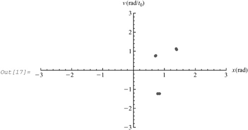
The Poincaré section has three dots and indicates periodic motion. (For an introduction to the Poincaré section, see [BG96] or [TM04].)
For another example, let a = 1/2, F = 1.15, and ω = 2/3:
In[18]:= a = 1/2; F = 1.15; ω = 2/3;
Also, choose the initial conditions x = 0.8 and y = 0.8.
For t from 0 to cycles(2π/ω), NDSolve solves Equations 4.3.3 and 4.3.7 together with the initial conditions:
In[19]:= cycles = 180;
         sol4 = NDSolve[{x'[t] == v[t],
            v'[t] == - Sin[x[t]] - a v[t] + F Cos[ω t], x[0] == 0.8, v[0] == 0.8},
            {x, v}, {t, 0, cycles(2 π/ω)}, MaxSteps → 200 000];
         steps = 30;
         points4 = Flatten[Table[{x[t], v[t]} /. sol4,
             {t, 0, cycles(2 π/ω), (1/steps) (2 π/ω)}], 1];
where we have generated a nested list of coordinates {x(t), v(t)}, with t ranging from 0 to cycles(2π/ω) in steps of size Δt = (1/steps)(2π/ω), for plotting the phase diagram and the Poincaré section. We must take computer solution of differential equations in chaotic dynamics with a grain of salt because sensitive dependence on initial conditions is a characteristic feature of chaos, and round-off error is an inherent limitation of numerical methods. (For further discussion, refer to [PJS92] and [Ras90].)
Let us plot the phase diagram with all the points translated back to the interval x = –π to +π and with the lines joining the points omitted for clarity:
In[23]:= newpoints4 = {reduce[ # [[1]]], # [[2]]} & /@ points4;
         ListPlot[newpoints4, AxesLabel → {"x (rad)","v (rad/t0 )"}]
Next, we construct the Poincaré section:
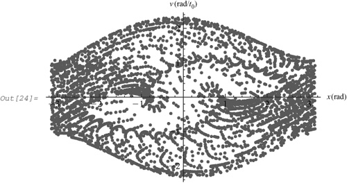
In[25]:= poincare4 = Table[newpoints4[[n]],
            {n, 1 + 20 steps, Length[newpoints4], steps}];
         ListPlot[poincare4, PlotRange → {{−4, 4}, {−4, 4}},
          AxesLabel → {"x (rad)","v (rad/t0 )"}]
The Poincaré section has a complex geometry that is characteristic of chaotic states.
We end this notebook with an animation showing the chaotic motion of the pendulum. The package ChaoticPendulum' containing the function Motion is included in Section 4.3.3.4. To use this package like a standard Mathematica package, follow the instructions at the end of Section 3.7.3.3. Motion[points, n, m] generates an animation of the pendulum. The first argument points is for the nested list of coordinates {x(ti), v(ti)} from the solution of the equation of motion, the second argument n is for the number of graphs of the pendulum to be plotted, and the third argument m is for the time increment. Only nonzero positive integers can be assumed by n and m. The time interval between two successive graphs is equal to m times the step size Δt previously specified. For given points and m, n has an upper limit
Ceiling [Length [points]/ m]Length [points] gives the number of elements in points, and Ceiling[x] is the least integer not smaller than x. Here is the number of elements in points4:
In[27]:= Length[points4]
Out[27]= 5401
Let us load the package ChaoticPendulum' and call the function Motion:
In[28]:= Needs["ChaoticPendulum'"]
         Motion[points4,1000,2]
To animate, click the Play button—that is, the one with the right pointer.
(* To use this package like a standard Mathematica package,
follow the instructions at the end of Section 3.7.3.3. * )


BeginPackage["ChaoticPendulum'"]

ChaoticPendulum::usage =
 "ChaoticPendulum' is a package for generating
   an animation of the pendulum."

Motion::usage =
 "Motion[points, n, m] generates an animation of the pendulum."
Begin["'Private'"]

Motion::badarg =
 "For the given nested list of coordinates and your choice
   of time increment, the maximum number of graphs that
   can be plotted is '1'. You requested '2' graphs."


Motion[points_ List, n_Integer?Positive, m_ Integer?Positive] := (
   list = Table[points[[i, 1]], {i, 1, Length[points], m}];
   x = Sin[list];
   y = -Cos[list];
   ListAnimate [
    Table [
     Show [
      Graphics[{Line[{{0, 0}, {x[[k]], y[[k]]}}],
        PointSize[0.05], Red, Point[{x[[k]], y[[k]]}]}],
      PlotRange → {{−1.25, 1.25}, {−1.25, 1.25}},
      AspectRatio → Automatic, Frame → True, FrameTicks → None,
      Background → Lighter[Blue, 0.5]], {k, n}]]
 ) /; n ≤ Ceiling[Length[points]/m]

Motion[points_ List,n_ Integer?Positive, m_ Integer? Positive] :=
 (Message[Motion::badarg, Ceiling[Length[points]/m], n] )/;
  n > Ceiling[Length[points]/m]

End[]

Protect[Motion]

EndPackage[]
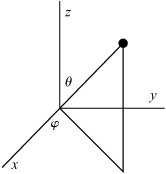
The spherical pendulum consists of a particle of mass m constrained by a rigid and massless rod to move on a sphere of radius R. With several choices of initial conditions for the pendulum, explore its motion.
We adopt a system of units in which m = 1, R = 1, and g = 1, where g is the magnitude of the acceleration due to gravity. Let θ and ϕ be the spherical coordinates of the particle, and let the fixed end of the rod be the origin, as in Figure 4.4.1. In terms of the spherical coordinates,
The gravitational potential energy relative to the horizontal plane is
Hence, the Lagrangian, T – V, can be expressed as
The Lagrange equations of motion give
Equations 4.4.4 and 4.4.5 together with the initial conditions θ00, ![]() , ϕ0, and
, ϕ0, and ![]() 0 completely specify the motion of the system. (For an introduction to Lagrangian mechanics, see [Sym71] or [TM04].)
0 completely specify the motion of the system. (For an introduction to Lagrangian mechanics, see [Sym71] or [TM04].)
We gain insight into the motion of the pendulum by recognizing that there are two constants of the motion: the angular momentum about the z-axis and the total energy. Since the coordinate ϕ is ignorable (i.e., it does not appear explicitly in the Lagrangian), the corresponding generalized momentum (also known as canonical momentum or conjugate momentum)
is a constant of the motion, as can be seen from Equation 4.4.5. The total energy
can also be shown to be a constant of the motion because the spherical pendulum is a natural system (i.e., the Lagrangian has the form T2 – V, where the kinetic energy T2 contains only terms quadratic in the generalized velocities and the potential energy V is velocity independent), the Lagrangian of which does not depend explicitly on time. (For a detailed discussion of the energy integral of the motion, see [CS60].) In terms of the angular momentum pϕ, Equations 4.4.4 and 4.4.5 can be written as
and Equation 4.4.7 can be put in the form

Let us define an effective potential
Equation 4.4.10 becomes
If pϕ = 0, Equations 4.4.8 and 4.4.9 are the equations of motion of a simple pendulum oscillating in a plane perpendicular to the xy plane. If pϕ = 0, Equation 4.4.9 indicates that, except for the two singularities at θ equals 0° and 180°, the sign of ![]() remains constant. Thus, the particle rotates about the z-axis. We obtain further insight into the motion of the pendulum by examining the effective potential curve in Figure 4.4.2. The effective potential rises to infinity at θ = 0° and θ = 180°. Therefore, these angles are inaccessible to the system unless the total energy is infinite because
remains constant. Thus, the particle rotates about the z-axis. We obtain further insight into the motion of the pendulum by examining the effective potential curve in Figure 4.4.2. The effective potential rises to infinity at θ = 0° and θ = 180°. Therefore, these angles are inaccessible to the system unless the total energy is infinite because ![]() 2 in Equation 4.4.12 cannot be negative. In general, the angle θ oscillates between two turning points θ1 and θ2, which are the roots of the equation
2 in Equation 4.4.12 cannot be negative. In general, the angle θ oscillates between two turning points θ1 and θ2, which are the roots of the equation
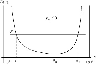
If E = U(θm), where θm is the angle for the minimum value of U(θ), these roots coincide and the particle rotates about the z-axis at the fixed angle θm and, from Equation 4.4.9, with constant ![]() .
.
In[1]:= ClearAll [";Global'*"]
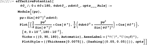
We begin with the definition of a function for plotting the effective potential together with the total energy. The first argument of the function is θ0 in degrees from 0° to 180°; the second argument, ![]() 0; and the third argument,
0; and the third argument, ![]() 0. Options, except
0. Options, except AxesLabel, PlotStyle, and Ticks, for passing to the Plot function may be specified after the third argument.
We now define the function that generates an animation of the spherical pendulum. The first argument of the function is θ0 in degrees from 0° to 180°; the second argument, ![]() 0 limited between –10 and 10; the third argument, ϕ0 in degrees from 0° to 360°; the fourth argument,
0 limited between –10 and 10; the third argument, ϕ0 in degrees from 0° to 360°; the fourth argument, ![]() 0 confined between –10 and 10; the fifth argument, the interval of time tmax restricted from 1 to 60 for the animation sequence; and the sixth argument, the number of frames nv generated with a minimum value of 2 and a computed default value of the integer closest to 3tmax. Options, with the exception of
0 confined between –10 and 10; the fifth argument, the interval of time tmax restricted from 1 to 60 for the animation sequence; and the sixth argument, the number of frames nv generated with a minimum value of 2 and a computed default value of the integer closest to 3tmax. Options, with the exception of PlotRange and BoxRatios, for passing to the Show function may be specified after these arguments. The construct of the function is explained in the body of the function with statements in the form (* comment *). The maximum possible values for tmax and nv depend on the available memory. With nv = 2, the function generates two frames: one for time t = 0 and another for t = tmax.
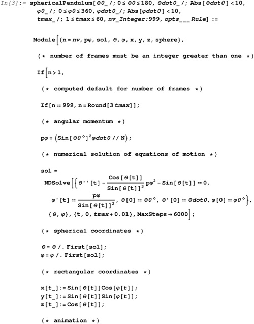
With the functions effectivePotential and sphericalPendulum, we are ready to explore the motion of the spherical pendulum with several choices of initial conditions.
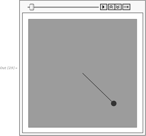
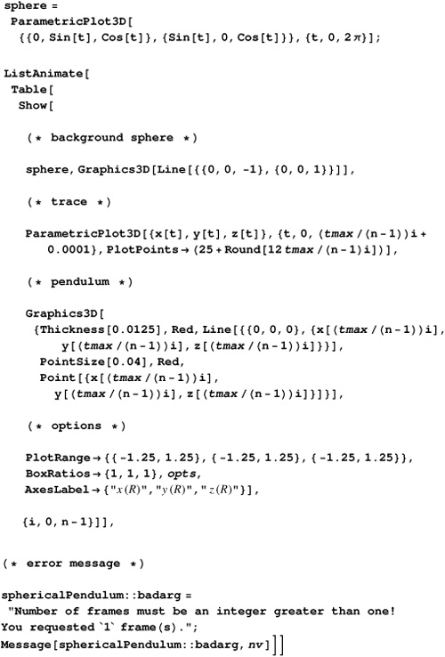
Since pϕ = 0, the spherical pendulum behaves as a simple pendulum. The function effective-Potential plots the effective potential together with the total energy:
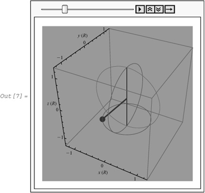
In[4]:= effectivePotential [120, 0, 0]
In the graph, the solid curve and the dashed line represent the effective potential and the total energy, respectively. The effective potential has a minimum at θ = 180°. The pendulum oscillates about this angle, and the turning point θ = 120° occurs at the intersection of the effective potential curve and the total energy line. The function sphericalPendulum generates the animation:
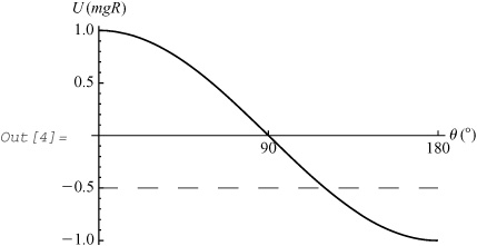
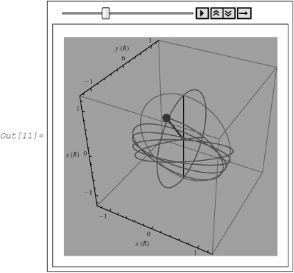
In[5]:= sphericalPendulum[120, 0, 45, 0, 27,
         Background → RGBColor[0.640004, 0.580004, 0.5]]
To animate, click the Play button—that is, the one with the right pointer. The curve traces the path of the particle from its initial position. In this case, the spherical pendulum behaves like a simple pendulum, as expected.
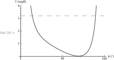
Let us plot the effective potential:
In[6]:= effectivePotential [135, 0, 21/4, PlotRange → {-0.5, 2.0}]
Since pϕ ≠ 0 and E = U(θm), the particle rotates uniformly in a horizontal circle about the z-axis. We now generate the animation:
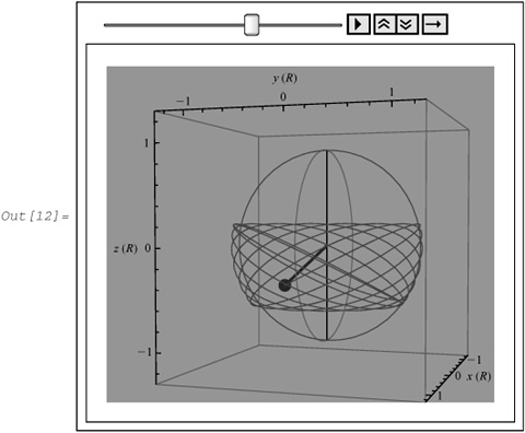
In[7]:= sphericalPendulum [135, 0, 90, 21/4, 31,
         Background → RGBColor[0.640004, 0.580004, 0.5]]
To animate, click the Play button. The pendulum indeed rotates uniformly about the z-axis.
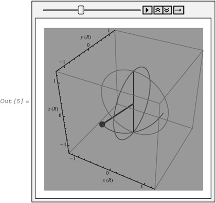
Again, we plot the effective potential:
In[8]:= effectivePotential [135, 2.5, 1.5 × 21/4, PlotRange → {-0.25, 4.0}]
The particle rotates about the z-axis while the angle θ oscillates between two turning points, θ ≈ 24° and θ ≈ 162°, which occur at the intersections of the effective potential curve and the energy line. Let us generate the animation:
In[9]:= sphericalPendulum [135, 2.5, 90, 1.5 × 21/4, 40,
         Background → RGBColor [0.640004, 0.580004, 0.5]]
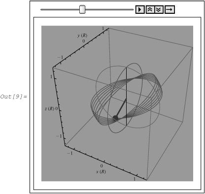
To animate, click the Play button. We see that the orbit of the pendulum rotates about an axis.
Once more, we plot the effective potential:
In[10]:= effectivePotential [120, 0.75, 2.0 × 21/4, PlotRange → {0, 4}]
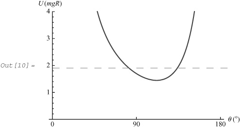
Here, the turning points for the angle θ are approximately 77° and 127°. We now generate the animation:
In[11]:= sphericalPendulum [120, 0.75, 90, 2.0 × 21/4,
          40, Background → RGBColor [0.640004, 0.580004, 0.5]]
To animate, click the Play button. We see that the motion of the pendulum is more complex than those of the preceding cases. As discussed previously, the angular momentum about the z-axis must remain constant during the motion.
It is instructive to observe the motion of the pendulum from another viewpoint.
In[12]:= sphericalPendulum [120, 0.75, 90, 2.0 × 21/4,
           40, Background → RGBColor [0.640004, 0.580004, 0.5],
           ViewPoint → {3.225, 1.018, 0.109}]
The path of the particle is clearly confined between two planes parallel to the xy plane; that is, the angle θ oscillates between two turning points.
In[13]:= ClearAll[effectivePotential, sphericalPendulum]
In this book, straightforward, intermediate-level, and challenging problems are unmarked, marked with one asterisk, and marked with two asterisks, respectively. For solutions to selected problems, see Appendix D.
1. | A physicist of mass mp (including paint) is about to paint her house. She places a uniform ladder of length L and mass mL against the house at an angle θ with respect to the ground. Being cautious, she decides to do a quick calculation to see how far up the ladder she can safely climb. Suppose there are rollers at the top of the ladder—that is, let the coefficient of (static) friction between the ladder and the house be zero, let the coefficient of (static) friction between the ladder and the ground be μ, and express the position of the physicist measured up the ladder from its base as fL. What fraction of the total length of the ladder does she calculate she can climb before the ladder slips, and what are the forces that the ground and the house exert on the ladder? Obtain numerical answers for the values mL = 9.50 kg, mp = 88.5 kg, μ = 0.55, θ = 50°, and g = 9.80 m/s2. (For solutions of this problem with MACSYMA, Maple, Mathcad, Mathematica, and Theorist, see [CDSTD92a].) |
2. | In Section 4.1.3, can we replace |
3. | Consider a body falling from rest near the surface of the earth. For a small heavy body with large terminal velocity, the effect of air resistance may be approximated by a frictional force proportional to the square of the speed. Determine the motion of the body. |
*4. | A projectile of mass m leaves the origin with a speed v0 at an angle θ0 from the horizontal. Assume that the effect of air resistance may be approximated by a frictional force –bv, where v is the velocity. (a) Obtain an equation for the trajectory—that is, y = f (x), where the x- and y-axes are along the horizontal and vertical directions, respectively. Hint: Use |
5. | Section 4.3.3.1 specified, for the plane pendulum, the initial conditions x = 0 and v = 2 – d, where d is a small number. (a) What is the significance of this choice of initial conditions? (b) Solve Equations 4.3.3 and 4.3.5 and plot the phase diagram for the initial conditions x = 0 and v = 2+ d, where d is again a small number. Explain the resulting phase diagram. (c) Repeat part (b) for the initial conditions x = 0 and v = 0. Is the resulting phase diagram what you expected? If not, why not? |
6. | Generate an animation of the periodic motion of a damped, driven pendulum with a = 0.2, F = 0.52, and ω = 0.694. Hint: See Section 4.3.3; discard points for the early cycles to avoid transient effects. |
*7. | Consider the Duffing–Holmes equation for the forced vibrations of a buckled elastic beam or the forced oscillations of a particle in a two-well potential: Solve the equation numerically, plot the phase diagram, and determine the Poincaré section for the following parameters: (a) γ = 0.15, ω = 0.8, F = 0.32; (b) γ = 0.15, ω = 0.8, F = 0.2; and (c) γ = 0.15, ω = 0.8, F = 0.15. |
8. | In Section 4.4.3, the first five arguments of the function |
*9. | Consider again Example 2.1.9 on the motion of a planet. (a) Plot the trajectory for the initial conditions x(0) = 1, y(0) = 0, x’(0) = 0, and y’(0) = 8. Since x’(0) = 0 and y’(0) = 8, should the orbit be a circle? Explain. (b) Plot the trajectory for x(0) = 1, y(0) = 0, x’(0) = –2.5, and y’(0) = 8. Should the foci of the ellipse be located on the x- or y-axis? Explain. (c) Find a set of initial conditions for which the orbit is a parabola. (d) Find a set of initial conditions for which the orbit is a hyperbola. Hint: See the discussion in Section 3.6.1. |
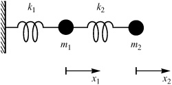
*10. | Two one-dimensional harmonic oscillators are attached as in Figure 4.5.1, where x1 and x2 are the displacements of m1 and m2, respectively. Each displacement is measured from the equilibrium position, and the direction to the right is positive. While m2 is held in place, m1 is moved to the left a distance a. At time t = 0, both masses are released. (a) Determine their subsequent motions. (b) What are the normal or characteristic frequencies of the system? (c) Plot x1(t) and x2(t)+2 on the same graph. (d) Is the motion of the system periodic? Hint: Use |
**11. | Write a function that generates an animation of the motion, as viewed from the laboratory frame, of a system of two identical masses under their mutual gravitational attraction. |