IN THIS CHAPTER

Defining imaginary and complex numbers

Writing complex solutions for quadratic equations

Determining complex solutions for polynomials

Mathematicians define real numbers as all the whole numbers, negative and positive numbers, fractions and decimals, radicals — anything you can think of to use in counting, graphing, and comparing amounts. Mathematicians introduced imaginary numbers when they couldn’t finish some problems without them. For example, when solving for roots of quadratic equations such as , you quickly discover that you can find no real answers. Using the quadratic formula, the solutions come out to be

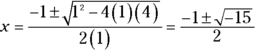
The equation has no real solution. So, instead of staying stuck there, mathematicians came up with something innovative. They made up a number and named it i.

The square root of can be replaced with the imaginary number i: . Furthermore, .

In this chapter, you find out how to create, work with, and analyze imaginary numbers and the complex expressions they appear in. Just remember to use your imagination!

Simplifying Powers of i

The powers of i (representing powers of imaginary numbers) follow the same mathematical rules as the powers of real numbers. The powers of i, however, have some neat features that set them apart from other numbers.

You can write all the powers of i as one of four different numbers: i, , 1, and ; all it takes is some simplifying of products, using the properties of exponents, to rewrite the powers of i:

• : Just plain old i.
• : From the definition of an imaginary number (see the introduction to this chapter).
• : Use the rule for exponents and then replace with . So, .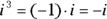
• : Because .
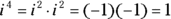• : Because .
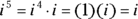• : Because .
• : Because .
• : Because .

Simplify the powers of i:

• : Because .
• : Because .

Every power of i where the exponent is a multiple of 4 is equal to 1. If the exponent is one value greater than a multiple of 4, the power of i is equal to i. An exponent that’s two more than a multiple of 4 results in ; and three more than a multiple of 4 as a power of i results in . So, all you need do to change the powers of i is figure out where the exponent is in relation to some multiple of four.

Getting More Complex with Complex Numbers

The imaginary number i is a part of the numbers called complex numbers, which arose after mathematicians established imaginary numbers. The standard form of complex numbers is , where a and b are real numbers, and is . The fact that is equal to and i is equal to is the foundation of the complex numbers.

Some examples of complex numbers include , , and 7i. In the last number, 7i, the value of a is 0.

Performing complex operations

You can add, subtract, multiply, and divide complex numbers — in a very careful manner. The rules used to perform operations on complex numbers look very much like the rules used for any algebraic expression, with two big exceptions:

• You simplify the powers of i.
• You don’t really divide complex numbers — you change the division problem to a multiplication problem.

Making addition and subtraction complex

When you add or subtract two complex numbers and together, you get the sum (difference) of the real parts and the sum (difference) of the imaginary parts:

Add and ; then subtract from .

Creating complex products

To multiply complex numbers, you have to treat the numbers like binomials and distribute both the terms of one complex number over the other:

Find the product of and .

You simplify the last term by replacing the with to give you . Then combine with the first term. Your result is , a complex number.

Performing complex division by multiplying by the conjugate

The complex thing about dividing complex numbers is that you don’t really divide. Instead of dividing, you do a multiplication problem — one that has the same answer as the division problem.

Describing the conjugate of a complex number

A complex number and its conjugate are and . The real part, the a, stays the same; the sign between the real and imaginary part changes. For example, the conjugate of is , and the conjugate of is .

The product of an imaginary number and its conjugate is a real number (no imaginary part) and takes the following form:

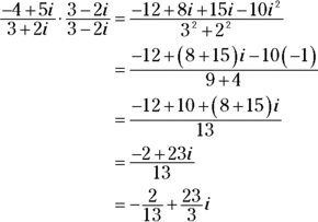
Dividing complex numbers

When a problem calls for you to divide one complex number by another, you write the problem as a fraction and then multiply by a fraction that has the conjugate of the denominator in both numerator and denominator.

Divide by .

Write the problem as a fraction. Then multiply the problem’s fraction by a second fraction that has the conjugate of in both numerator and denominator.

Simplifying reluctant radicals

Until mathematicians defined imaginary numbers, many problems had no answers because the answers involved square roots of negative numbers. After the definition of an imaginary number, , came into being, the problems involving square roots of negative numbers were solved.

To simplify the square root of a negative number, you write the square root as the product of square roots and simplify: .

Simplify .

First, split up the radical into the square root of and the square root of the rest of the number, and then simplify by factoring out perfect squares:

By convention, you write the previous solution as .

Unraveling Complex Solutions in Quadratic Equations

You can always solve quadratic equations with the quadratic formula. It may be easier to solve quadratic equations by factoring, but when you can’t factor, the formula comes in handy. Until mathematicians began recognizing imaginary numbers, however, they couldn’t complete many results of the quadratic formula. Whenever a negative value appeared under a radical, the equation stumped the mathematicians.

The modern world of imaginary numbers to the rescue! Now quadratics with complex answers have results to show.

Solve the quadratic equation .

Using the quadratic formula, you let , , and :

Investigating Polynomials with Complex Roots

Polynomials are functions whose graphs are nice, smooth curves that may or may not cross the x-axis. If the degree (or highest power) of a polynomial is an odd number, its graph must cross the x-axis, and it must have a real root or solution. When solving equations formed by setting polynomials equal to 0, you plan ahead as to how many solutions you can expect to find. The highest power tells you the maximum number of solutions you can find. If the solutions are real, then the curve either crosses the x-axis or touches it. If any solutions are complex, then the number of crossings or touches is decreased by the number of complex roots.

Making use of complex zeros

The polynomial function has two real roots and two complex roots. According to Descartes’ rule of signs, the function could’ve contained as many as four real roots (suggested by the rational root theorem). You can determine the number of complex roots in two different ways: by factoring the polynomial or by looking at the graph of the function.

The polynomial function factors into . The first two factors give you real roots, or x-intercepts. When you set equal to 0, you get the intercept (2, 0). When you set equal to 0, you get the intercept . Setting the last factor, , equal to 0 doesn’t give you a real root.

But you can also tell that the polynomial function has complex roots by looking at its graph. You can’t tell what the roots are, but you can see that the graph has some. If you need the values of the roots, you can resort to using algebra to solve for them. Figure 12-1 shows the graph of the example function, . You can see the two x-intercepts, which represent the two real zeros. You also see the graph flattening on the left.

Figure 12-2 can tell you plenty about the number of real zeros and complex zeros the graph of the polynomial has … before you ever see the equation it represents.

The polynomial in Figure 12-2 appears to have one real zero and several complex zeros. Do you see how it changes direction all over the place under the x-axis? These changes indicate the presence of complex zeros. The graph represents the polynomial function . The function has four complex zeros — two complex (conjugate) pairs — and one real zero (when ).