Chapter Thirteen
Balanced Trees
THE BST ALGORITHMS in the previous chapter work well for a wide variety of applications, but they do have the problem of bad worst-case performance. What is more, it is embarrassingly true that the bad worst case for the standard BST algorithm, like that for quicksort, is one that is likely to occur in practice if the user of the algorithm is not watching for it. Files already in order, files with large numbers of duplicate keys, files in reverse order, files with alternating large and small keys, or files with any large segment having a simple structure can all lead to quadratic BST construction times and linear search times.
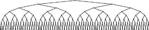
In the ideal case, we could keep our trees perfectly balanced, like the tree depicted in Figure 13.1. This structure corresponds to binary search and therefore allows us to guarantee that all searches can be completed in less than lg N + 1 comparisons, but is expensive to maintain for dynamic insertions and deletions. The search performance guarantee holds for any BST for which all the external nodes are on the bottom one or at most two levels, and there are many such BSTs, so we have some flexibility in arranging for our tree to be balanced. If we are satisfied with near-optimal trees, then we can have even more flexibility. For example, there are a great many BSTs of height less than 2 lg N. If we relax our standard but can guarantee that our algorithms build only such BSTs, then we can provide the protection against bad worst-case performance that we would like to have in practical applications in a dynamic data structure. As a side benefit, we get better average-case performance, as well.
Figure 13.1 A large BST that is perfectly balanced The external nodes in this BST all fall on one of two levels, and the number of comparisons for any search is the same as the number of comparisons that would be used by binary search for the same key (if the items were in an ordered array). The goal of a balanced-tree algorithm is to keep a BST as close as possible to being as well balanced as this one, while still supporting efficient dynamic insertion, deletion, and other dictionary ADT operations.
One approach to producing better balance in BSTs is periodically to rebalance them explicitly. Indeed, we can balance most BSTs completely in linear time, using the recursive method shown in Program 13.1 (see Exercise 13.4). Such rebalancing is likely to improve performance for random keys, but does not provide guarantees against quadratic worst-case performance in a dynamic symbol table. On the one hand, the insertion time for a sequence of keys between rebalancing operations can grow quadratic in the length of the sequence; on the other hand, we do not want to rebalance huge trees frequently, because each rebalancing operation costs at least linear time in the size of the tree. This tradeoff makes it difficult to use global rebalancing to guarantee fast performance in dynamic BSTs. All the algorithms that we will consider, as they walk through the tree, do incremental, local operations that collectively improve the balance of the whole tree, yet they never have to walk through all the nodes in the way that Program 13.1 does.
The problem of providing guaranteed performance for symbol-table implementations based on BSTs gives us an excellent forum for examining precisely what we mean when we ask for performance guarantees. We shall see solutions to this problem that are prime examples of each of the three general approaches to providing performance guarantees in algorithm design: we can randomize, amortize, or optimize. We now consider each of these approaches briefly, in turn.
A randomized algorithm introduces random decision making into the algorithm itself, to reduce dramatically the chance of a worst-case scenario (no matter what the input). We have already seen a prime example of this arrangement, when we used a random element as the partitioning element in quicksort. In Sections 13.1 and 13.5, we shall examine randomized BSTs and skip lists—two simple ways to use randomization in symbol-table implementations to give efficient implementations of all the symbol-table ADT operations. These algorithms are simple and are broadly applicable, but went undiscovered for decades (see reference section). The analysis that proves these algorithms to be effective is not elementary, but the algorithms are simple to understand, to implement, and to put to practical use.
An amortization approach is to do extra work at one time to avoid more work later, to be able to provide guaranteed upper bounds on the average per-operation cost (the total cost of all operations divided by the number of operations). In Section 13.2, we shall examine splay BSTs, a variant of BSTs that we can use to provide such guarantees for symbol-table implementations. The development of this method was one impetus for the development of the concept of amortization (see reference section). The algorithm is a straightforward extension of the root insertion method that we discussed in Chapter 12, but the analysis that proves the performance bounds is sophisticated.
An optimization approach is to take the trouble to provide performance guarantees for every operation. Various methods have been developed that take this approach, some dating back to the 1960s. These methods require that we maintain some structural information in the trees, and programmers typically find the algorithms cumbersome to implement. In this chapter, we shall examine two simple abstractions that not only make the implementation straightforward, but also lead to near-optimal upper bounds on the costs.
After examining implementations of symbol-table ADTs with guaranteed fast performance using each of these three approaches, we conclude the chapter with a comparison of performance characteristics. Beyond the differences suggested by the differing natures of the performance guarantees that each of the algorithms provides, the methods each carry a (relatively slight) cost in time or space to provide those guarantees; the development of a truly optimal balanced-tree ADT is still a research goal. Still, the algorithms that we consider in this chapter are all important ones that can provide fast implementations of search and insert (and several other symbol-table ADT operations) in dynamic symbol tables for a variety of applications.
Exercises
![]() 13.1 Implement an efficient function that rebalances BSTs that do not have a count field in their nodes.
13.1 Implement an efficient function that rebalances BSTs that do not have a count field in their nodes.
13.2 Modify the standard BST insertion function in Program 12.8 to use Program 13.1 to rebalance the tree each time that the number of items in the symbol table reaches a power of 2. Compare the running time of your program with that of Program 12.8 for the tasks of (i) building a tree from N random keys and (ii) searching for N random keys in the resulting tree, for N = 103, 104, 105, and 106.
13.3 Estimate the number of comparisons used by your program from Exercise 13.2 when inserting an increasing sequence of N keys into a symbol table.
![]()
![]() 13.4 Show that Program 13.1 runs in time proportional to
13.4 Show that Program 13.1 runs in time proportional to NlogN for a degenerate tree. Then give as weak a condition on the tree as you can that implies that the program runs in linear time.
13.5 Modify the standard BST insertion function in Program 12.8 to partition about the median any node encountered that has less than one-quarter of its nodes in one of its subtrees. Compare the running time of your program with that of Program 12.8 for the tasks of (i) building a tree from N random keys, and (ii) searching for N random keys in the resulting tree, for N = 103, 104, 105, and 106.
13.6 Estimate the number of comparisons used by your program from Exercise 13.5 when inserting an increasing sequence of N keys into a symbol table.
![]() 13.7 Extend your implementation in Exercise 13.5 to rebalance in the same way while performing the remove function. Run experiments to determine whether the height of the tree grows as a long sequence of alternating random insertions and deletions are made in a random tree of N nodes, for N = 10, 100, and 1000, and for N2 insertion–deletion pairs for each N.
13.7 Extend your implementation in Exercise 13.5 to rebalance in the same way while performing the remove function. Run experiments to determine whether the height of the tree grows as a long sequence of alternating random insertions and deletions are made in a random tree of N nodes, for N = 10, 100, and 1000, and for N2 insertion–deletion pairs for each N.
13.1 Randomized BSTs
To analyze the average-case performance costs for binary search trees, we made the assumption that the items are inserted in random order (see Section 12.6). The primary consequence of this assumption in the context of the BST algorithm is that each node in the tree is equally likely to be the one at the root, and this property also holds for the subtrees. Remarkably, it is possible to introduce randomness into the algorithm so that this property holds without any assumptions about the order in which the items are inserted. The idea is simple: When we insert a new node into a tree of N nodes, the new node should appear at the root with probability 1/(N + 1), so we simply make a randomized decision to use root insertion with that probability. Otherwise, we recursively use the method to insert the new record into the left subtree if the record’s key is less than the key at the root, and into the right subtree if the record’s key is greater.Program 13.2 is an implementation of this method.
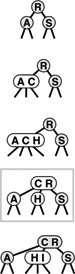
Viewed nonrecursively, doing randomized insertion is equivalent to performing a standard search for the key, making a randomized decision at every step whether to continue the search or to terminate it and do root insertion. Thus, the new node could be inserted anywhere on its search path, as illustrated in Figure 13.2. This simple probabilistic combination of the standard BST algorithm with the root insertion method gives guaranteed performance in a probabilistic sense.
Property 13.1 Building a randomized BST is equivalent to building a standard BST from a random initial permutation of the keys. We use about 2N ln N comparisons to construct a randomized BST with N items (no matter in what order the items are presented for insertion), and about 2 ln N comparisons for searches in such a tree.
Each element is equally likely to be the root of the tree, and this property holds for both subtrees, as well. The first part of this statement is true by construction, but a careful probabilistic argument is needed to show that the root insertion method preserves randomness in the subtrees (see reference section). ![]()
The distinction between average-case performance for randomized BSTs and for standard BSTs is subtle, but essential. The average costs are the same (though the constant of proportionality is slightly higher for randomized trees), but for standard trees the result depends on the assumption that the items are presented for insertion in a random ordering of their keys (all orderings equally likely). This assumption is not valid in many practical applications, and therefore the significance of the randomized algorithm is that it allows us to remove the assumption, and to depend instead on the laws of probability and randomness in the random-number generator. If the items are inserted with their keys in order, or in reverse order, or any order whatever, the BST will still be random.
Figure 13.2 Insertion into a randomized BST The final position of a new record in a randomized BST may be anywhere on the record’s search path, depending on the outcome of randomized decisions made during the search. This figure shows each of the possible final positions for a record with key F when the record is inserted into a sample tree (top).
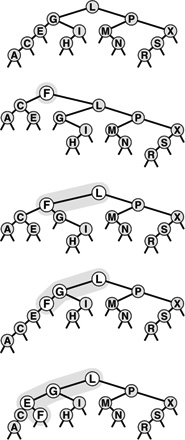
Figure 13.3 depicts the construction of a randomized tree for an example set of keys. Since the decisions made by the algorithm are randomized, the sequence of trees is likely to be different each time that we run the algorithm. Figure 13.4 shows that a randomized tree constructed from a set of items with keys in increasing order looks to have the same properties as a standard BST constructed from randomly ordered items (cf. Figure 12.8).
There is still a chance that the random number generator could lead to the wrong decision at every opportunity, and thus leave us with poorly balanced trees, but we can analyze this chance mathematically and prove it to be vanishingly small.
Property 13.2 The probability that the construction cost of a randomized BST is more than a factor of α times the average is less than e-α.
This result and similar ones with the same character are implied by a general solution to probabilistic recurrence relations that was developed by Karp in 1995 (see reference section).![]()
For example, it takes about 2.3 million comparisons to build a randomized BST of 100,000 nodes, but the probability that the number of comparisons will be more than 23 million is much less than 0.01 percent. Such a performance guarantee is more than adequate for meeting the practical requirements of processing real data sets of this size. When using a standard BST for such a task, we cannot provide such a guarantee: for example, we are subject to performance problems if there is significant order in the data, which is unlikely in random data, but certainly would not be unusual in real data, for a host of reasons.
A result analogous to Property 13.2 also holds for the running time of quicksort, by the same argument. But the result is more important here, because it also implies that the cost of searching in the tree is close to the average. Regardless of any extra costs in constructing the trees, we can use the standard BST implementation to perform search operations, with costs that depend only on the shape of the trees, and no extra costs at all for balancing. This property is important in typical applications, where search operations are far more numerous than are any others. For example, the 100,000-node BST described in the previous paragraph might hold a telephone directory, and might be used for millions of searches. We can be nearly certain that each search will be within a small constant factor of the average cost of about 23 comparisons, and, for practical purposes, we do not have to worry about the possibility that a large number of searches would cost close to 100,000 comparisons, whereas with standard BSTs, we would need to be concerned.
Figure 13.3 Construction of a randomized BST This sequence depicts the insertion of the keys A B C D E F G H I into an initially empty BST, with randomized insertion. The tree at the bottom appears to have been built with the standard BST algorithm, with the same keys inserted in random order.
One of the main drawbacks to randomized insertion is the cost of generating random numbers at every node during every insertion. A high-quality system-supported random number generator might work hard to produce pseudo-random numbers with more randomness than randomized BSTs require, so constructing a randomized BST might be slower than constructing a standard BST in certain practical situations (for example, if the assumption that the items are in random order is valid). As we did with quicksort, we can reduce this cost by using numbers that are less than perfectly random, but that are cheap to generate and are sufficiently similar to random numbers that they achieve the goal of avoiding the bad worst case for BSTs for key insertion sequences that are likely to arise in practice (see Exercise 13.14).
Another potential drawback of randomized BSTs is that they need to have a field in each node for the number of nodes in that node’s subtree. The extra space required for this field may be a liability for large trees. On the other hand, as we discussed in Section 12.9, this field may be needed for other reasons—for example, to support the select operation, or to provide a check on the integrity of the data structure. In such cases, randomized BSTs incur no extra space cost, and are an attractive choice.
The basic guiding principle of preserving randomness in the trees also leads to efficient implementations of the remove, join, and other symbol-table ADT operations, still producing random trees.
To join an N-node tree with an M-node tree, we use the basic method from Chapter 12, except that we make a randomized decision to choose the root based on reasoning that the root of the combined tree must come from the N-node tree with probability N/(M + N) and from the M-node tree with probability M/(M + N).Program 13.3 is an implementation of this operation.
In the same way, we replace the arbitrary decision in the remove algorithm by a randomized one, as shown in Program 13.4. This method corresponds to an option that we did not consider for deleting nodes in standard BSTs because it would seem—in the absence of randomization—to lead to unbalanced trees (see Exercise 13.21).
Figure 13.4 A large randomized BST This BST is the result of inserting 200 keys in increasing order into an initially empty tree, using randomized insertion. The tree appears to have been built from randomly ordered keys (see Figure 12.8).
Property 13.3 Making a tree with an arbitrary sequence of randomized insert, remove, and join operations is equivalent to building a standard BST from a random permutation of the keys in the tree.
As it is for Property 13.1, a careful probabilistic argument is needed to establish this fact (see reference section). ![]()
Proving facts about probabilistic algorithms requires having a good understanding of probability theory, but understanding these proofs is not necessarily a requirement for programmers using the algorithms. A careful programmer will check claims such as Property 13.3 no matter how they are proved (to check, for example, the quality of the random-number generator or other properties of the implementation), and therefore can use these methods with confidence. Randomized BSTs are perhaps the easiest way to support a full symbol-table ADT with near-optimal performance guarantees; they are therefore useful for many practical applications.
Exercises
![]() 13.8 Draw the randomized BST that results when you insert items with the keys E A S Y Q U T I O N in that order into an initially empty tree, assuming a bad randomization function that results in the root insertion option being taken whenever the tree size is odd.
13.8 Draw the randomized BST that results when you insert items with the keys E A S Y Q U T I O N in that order into an initially empty tree, assuming a bad randomization function that results in the root insertion option being taken whenever the tree size is odd.
13.9 Write a driver program that performs the following experiment 1000 times, for N = 10 and 100: Insert items with keys 0 through N - 1 (in that order) into an initially empty randomized BST using Program 13.2. Then print, for each N, the χ2 statistic for the hypothesis that each key falls at the root with probability 1/N (see Exercise 14.5).
![]() 13.10 Give the probability that F lands in each of the positions depicted in Figure 13.2.
13.10 Give the probability that F lands in each of the positions depicted in Figure 13.2.
13.11 Write a program to compute the probability that a randomized insertion ends at one of the internal nodes in a given tree, for each of the nodes on the search path.
13.12 Write a program to compute the probability that a randomized insertion ends at one of the external nodes of a given tree.
![]() 13.13 Implement a nonrecursive version of the randomized insertion function in Program 13.2.
13.13 Implement a nonrecursive version of the randomized insertion function in Program 13.2.
13.14 Draw the randomized BST that results when you insert items with the keys E A S Y Q U T I O N in that order into an initially empty tree, using a version of Program 13.2 where you replace the expression involving rand() with the test (111 % h->N) == 3 to decide to switch to root insertion.
13.15 Do Exercise 13.9 for a version of Program 13.2 where you replace the expression involving rand() with the test (111 % h->N) == 3 to decide to switch to root insertion.
13.16 Show the sequence of randomized decisions that would result in the keys E A S Y Q U T I O N being built into a degenerate tree (keys in order, left links null). What is the probability that this event will happen?
13.17 Could every BST containing the keys EASYQUTION be constructed by some sequence of randomized decisions when those keys are inserted in that order into an initially empty tree? Explain your answer.
13.18 Run empirical studies to compute the average and standard deviation of the number of comparisons used for search hits and for search misses in a randomized BST built by inserting N random keys into an initially empty tree, for N = 103, 104, 105, and 106.
![]() 13.19 Draw the BST that results from using Program 13.4 to delete the Q from your tree in Exercise 13.14, using the test
13.19 Draw the BST that results from using Program 13.4 to delete the Q from your tree in Exercise 13.14, using the test (111 % (a->N + b->N)) < a->N to decide to join with a at the root.
13.20 Draw the BST that results when you insert items with the keys E A S Y into one initially empty tree, and items with the keys Q U E S T I O N into another initially empty tree, then combine the result, using Program 13.3 with the test described in Exercise 13.19.
13.21 Draw the BST that results when you insert items with the keys EASY Q U T I O N in that order into an initially empty tree, then use Program 13.4 to delete the Q, assuming a bad randomization function that always returns 0.
13.22 Run experiments to determine how the height of a BST grows as a long sequence of alternating random insertions and deletions using Programs 13.2 and 13.3 is made in a tree of N nodes, for N = 10, 100, and 1000, and for N2 insertion–deletion pairs for each N.
![]() 13.23 Compare your results from Exercise 13.22 with the result of deleting and reinserting the largest key in a random tree of
13.23 Compare your results from Exercise 13.22 with the result of deleting and reinserting the largest key in a random tree of N nodes using Programs 13.2 and 13.3, for N = 10, 100, and 1000, and for N2 insertion–deletion pairs for each N.
13.24 Instrument your program from Exercise 13.22 to determine the average number of calls to rand() that it makes per item deleted.
13.2 Splay BSTs
In the root-insertion method of Section 12.8, we accomplished our primary objective of bringing the newly inserted node to the root of the tree by using left and right rotations. In this section, we examine how we can modify root insertion such that the rotations balance the tree in a certain sense, as well.
Rather than considering (recursively) the single rotation that brings the newly inserted node to the top of the tree, we consider the two rotations that bring the node from a position as one of the grandchildren of the root up to the top of the tree. First, we perform one rotation to bring the node to be a child of the root. Then, we perform another rotation to bring it to the root. There are two essentially different cases, depending on whether or not the two links from the root to the node being inserted are oriented in the same way. Figure 13.5 shows the case where the orientations are different; the left part of Figure 13.6 shows the case where the orientations are the same. Splay BSTs are based on the observation that there is an alternative way to proceed when the links from the root to the node being inserted are oriented in the same way: Simply perform two rotations at the root, as shown at the right in Figure 13.6.
Splay insertion brings newly inserted nodes to the root using the transformations shown in Figure 13.5 (standard root insertion when the links from the root to the grandchild on the search path have different orientation) and on the right in Figure 13.6 (two rotations at the root when the links from the root to the grandchild on the search path have the same orientation). The BSTs built in this way are splay BSTs.Program 13.5 is a recursive implementation of splay insertion; Figure 13.7 depicts an example of a single insertion, and Figure 13.8 shows the construction process for a sample tree. The difference between splay insertion and standard root insertion may
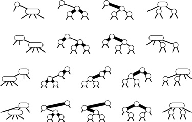
Figure 13.5 Double rotation in a BST (orientations different) In this sample tree (top), a left rotation at G followed by a right rotation at L brings I to the root (bottom). These rotations might complete a standard or splay BST root-insertion process.
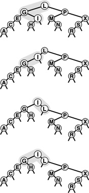
Figure 13.6 Double rotation in a BST (orientations alike) We have two options when both links in a double rotation are oriented in the same direction. With the standard root insertion method, we perform the lower rotation first (left); with splay insertion, we perform the higher rotation first (right).
seem inconsequential, but it is quite significant: the splay operation eliminates the quadratic worst case that is the primary liability of standard BSTs.
Property 13.4 The number of comparisons used when a splay BST is built from N insertions into an initially empty tree is O(N lg N).
This bound is a consequence of Property 13.5, a stronger property that we will consider shortly. ![]()
The constant implied in the O-notation is 3. For example, it always takes less than 5 million comparisons to build a BST of 100,000 nodes using splay insertion. This result does not guarantee that the resulting search tree will be well-balanced, and does not guarantee that each operation will be efficient, but the implied guarantee on the total running time is significant, and the actual running time that we observe in practice is likely to be lower still.
When we insert a node into a BST using splay insertion, we not only bring that node to the root, but also bring the other nodes that we encounter (on the search path) closer to the root. Precisely, the rotations that we perform cut in half the distance from the root to any node that we encounter. This property also holds if we implement the search operation such that it performs the splay transformations during the search. Some paths in the trees do get longer: If we do not access nodes on those paths, that effect is of no consequence to us. If we do access nodes on a long path, it becomes one-half as long after we do so; thus, no one path can build up high costs.
Property 13.5 The number of comparisons required for any sequence of M insert or search operations in an N-node splay BST is O((N + M) lg(N + M)).
The proof of this result, by Sleator and Tarjan in 1985, is a classic example of amortized analysis of algorithms (see reference section). We will examine it in detail in Part 8. ![]()
Property 13.5 is an amortized performance guarantee: We guarantee not that each operation is efficient, but rather that the average cost of all the operations performed is efficient. This average is not a probabilistic one; rather, we are stating that the total cost is guaranteed to be low. For many applications, this kind of guarantee suffices, but it may not be adequate for some other applications. For example, we cannot provide guaranteed response times for each operation when using splay BSTs, because some operations could take linear time. If an operation does take linear time, then we are guaranteed that other operations will be that much faster, but that may be no consolation to the customer who had to wait.
The bound given in Property 13.5 is a worst-case bound on the total cost of all operations: As is typical with worst-case bounds, it may be much higher than the actual costs. The splaying operation brings recently accessed elements closer to the top of the tree; therefore, this method is attractive for search applications with nonuniform access patterns—particularly applications with a relatively small, even if slowly changing, working set of accessed items.
Figure 13.7 Splay insertion This figure depicts the result (bottom) of inserting a record with key D into the sample tree at top, using splay root insertion. In this case, the insertion process consists of a left-right double rotation followed by a right-right double rotation (from the top).
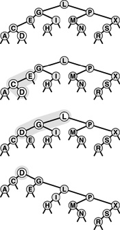
Figure 13.9 gives two examples that show the effectiveness of the splay-rotation operations in balancing the trees. In these figures, a degenerate tree (built via insertion of items in order of their keys) is brought into relatively good balance by a small number of search operations.
If duplicate keys are maintained in the tree, then the splay operation can cause items with keys equal to the key in a given node to fall on both sides of that node (see Exercise 13.38). This observation tells us that we cannot find all items with a given key as easily as we can for standard binary search trees. We must check for duplicates in both subtrees, or use some alternative method to work with duplicate keys, as discussed in Chapter 12.
Exercises
![]() 13.25 Draw the splay BST that results when you insert items with the keys E A S Y Q U T I O N in that order into an initially empty tree, using splay insertion.
13.25 Draw the splay BST that results when you insert items with the keys E A S Y Q U T I O N in that order into an initially empty tree, using splay insertion.
![]() 13.26 How many tree links must be changed for a double rotation? How many are actually changed for each of the double rotations in Program 13.5?
13.26 How many tree links must be changed for a double rotation? How many are actually changed for each of the double rotations in Program 13.5?
![]() 13.27 Add an implementation of search, with splaying, to Program 13.5.
13.27 Add an implementation of search, with splaying, to Program 13.5.
![]() 13.28 Implement a nonrecursive version of the splay insertion function in Program 13.5.
13.28 Implement a nonrecursive version of the splay insertion function in Program 13.5.
![]() 13.29 Use your driver program from Exercise 12.30 to determine the effectiveness of splay BSTs as self-organizing search structures by comparing them with standard BSTs for the search query distributions defined in Exercises 12.31 and 12.32.
13.29 Use your driver program from Exercise 12.30 to determine the effectiveness of splay BSTs as self-organizing search structures by comparing them with standard BSTs for the search query distributions defined in Exercises 12.31 and 12.32.
![]() 13.30 Draw all the structurally different BSTs that can result when you insert
13.30 Draw all the structurally different BSTs that can result when you insert N keys into an initially empty tree using splay insertion, for 2 ≤ N ≤ 7.
![]() 13.31 Find the probability that each of the trees in Exercise 13.30 is the result of inserting N random distinct elements into an intially empty tree.
13.31 Find the probability that each of the trees in Exercise 13.30 is the result of inserting N random distinct elements into an intially empty tree.
![]() 13.32 Run empirical studies to compute the average and standard deviation of the number of comparisons used for search hits and for search misses in a BST built by insertion of
13.32 Run empirical studies to compute the average and standard deviation of the number of comparisons used for search hits and for search misses in a BST built by insertion of N random keys into an initially empty tree with splay insertion, for N = 103, 104, 105, and 106. You do not need to do any searches: Just build the trees and compute their path lengths. Are splay BSTs more nearly balanced than random BSTs, less so, or the same?
13.33 Extend your program for Exercise 13.32 to do N random searches (they most likely will be misses) with splaying in each tree constructed. How does splaying affect the average number of comparisons for a search miss?
13.34 Instrument your programs for Exercises 13.32 and 13.33 to measure running time, rather than just to count comparisons. Run the same experiments. Explain any changes in the conclusions that you draw from the empirical results.
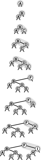
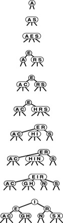
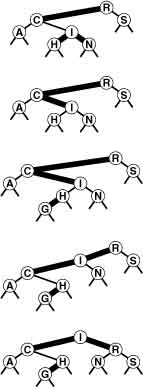
Figure 13.8 Splay BST construction This sequence depicts the insertion of records with keys A S E R C H I N G into an initially empty tree using splay insertion.
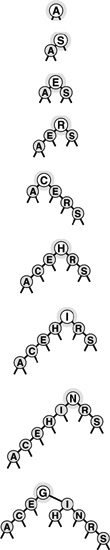
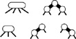
Figure 13.9 Balancing of a worst-case splay tree with searches
Inserting keys in sorted order into an initially empty tree using splay insertion takes only a constant number of steps per insertion, but leaves an unbalanced tree, shown at the top on the left and on the right. The sequence on the left shows the result of searching (with splaying) for the smallest, second-smallest, third-smallest, and fourth-smallest keys in the tree. Each search halves the length of the path to the search key (and most other keys in the tree). The sequence on the right shows the same worst-case starting tree being balanced by a sequence of random search hits. Each search halves the number of nodes on its path, reducing the length of search paths for many other nodes in the tree. Collectively, a small number of searches improves the tree balance substantially.
13.35 Compare splay BSTs with standard BSTs for the task of building an index from a piece of real-world text that has at least 1 million characters. Measure the time taken to build the index and the average path lengths in the BSTs.
13.36 Empirically determine the average number of comparisons for search hits in a splay BST built by inserting random keys, for N = 103, 104, 105, and 106.
13.37 Run empirical studies to test the idea of using splay insertion, instead of standard root insertion, for randomized BSTs.
![]() 13.38 Draw the splay BST that results when you insert items with the keys 0 0 0 0 0 0 0 0 0 0 0 0 1 in that order into an initially empty tree.
13.38 Draw the splay BST that results when you insert items with the keys 0 0 0 0 0 0 0 0 0 0 0 0 1 in that order into an initially empty tree.
13.3 Top-Down 2-3-4 Trees
Despite the performance guarantees that we can provide with randomized BSTs and with splay BSTs, both still admit the possibility that a particular search operation could take linear time. They therefore do not help us answer the fundamental question for balanced trees: Is there a type of BST for which we can guarantee that each and every insert and search operation will be logarithmic in the size of the tree? In this section and Section 13.4, we consider an abstract generalization of BSTs and an abstract representation of these trees as a type of BST that allows us to answer this question in the affirmative.
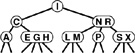
Figure 13.10 A 2-3-4 tree This figure depicts a 2-3-4 tree that contains the keys A S R C H I N G E X M P L. We can find a key in such a tree by using the keys in the node at the root to find a link to a subtree, then continuing recursively. For example, to search for P in this tree, we would follow the right link from the root, since P is larger than I, follow the middle link from the right child of the root, since P is between N and R, then terminate the successful search at the 2-node containing the P.
To guarantee that our BSTs will be balanced, we need flexibility in the tree structures that we use. To get this flexibility, let us assume that the nodes in our trees can hold more than one key. Specifically, we will allow 3-nodes and 4-nodes, which can hold two and three keys, respectively. A 3-node has three links coming out of it: one for all items with keys smaller than both its keys, one for all items with keys in between its two keys, and one for all items with keys larger than both its keys. Similarly, a 4-node has four links coming out of it: one for each of the intervals defined by its three keys. The nodes in a standard BST could thus be called 2-nodes: one key, two links. Later, we shall see efficient ways to define and implement the basic operations on these extended nodes; for now, let us assume that we can manipulate them conveniently, and see how they can be put together to form trees.
Definition 13.1 A 2-3-4 search tree is a tree that either is empty or comprises three types of nodes: 2-nodes, with one key, a left link to a tree with smaller keys, and a right link to a tree with larger keys; 3-nodes, with two keys, a left link to a tree with smaller keys, a middle link to a tree with key values between the node’s keys and a right link to a tree with larger keys; and 4-nodes, with three keys and four links to trees with key values defined by the ranges subtended by the node’s keys.
Definition 13.2 A balanced 2-3-4 search tree is a 2-3-4 search tree with all links to empty trees at the same distance from the root.
In this chapter, we shall use the term 2-3-4 tree to refer to balanced 2-3-4 search trees (it denotes a more general structure in other contexts). Figure 13.10 depicts an example of a 2-3-4 tree. The search algorithm for keys in such a tree is a generalization of the search algorithm for BSTs. To determine whether a key is in the tree, we compare it against the keys at the root: If it is equal to any of them, we have a search hit, otherwise, we follow the link from the root to the subtree corresponding to the set of key values containing the search key, and recursively search in that tree. There are a number of ways to represent 2-, 3-, and 4-nodes and to organize the mechanics of finding the proper link; we defer discussing these solutions until Section 13.4, where we shall discuss a particularly convenient arrangement.
To insert a new node in a 2-3-4 tree, we could do an unsuccessful search and then hook on the node, as we did with BSTs, but the new tree would not be balanced. The primary reason that 2-3-4 trees are important is that we can do insertions and still maintain perfect balance in the tree, in every case. For example, it is easy to see what to do if the node at which the search terminates is a 2-node: We just turn the node into a 3-node. Similarly, if the search terminates at a 3-node, we just turn the node into a 4-node. But what should we do if the search terminates at a 4-node? The answer is that we can make room for the new key while maintaining the balance in the tree, by first splitting the 4-node into two 2-nodes, passing the middle key up to the node’s parent. These three cases are illustrated in Figure 13.11.
Now, what do we do if we need to split a 4-node whose parent is also a 4-node? One method would be to split the parent also, but the grandparent could also be a 4-node, and so could its parent, and so forth—we could wind up splitting nodes all the way back up the tree. An easier approach is to make sure that the search path will not end at a 4-node, by splitting any 4-node we see on the way down the tree.
Figure 13.11 Insertion into a 2-3-4 tree A 2-3-4 tree consisting only of 2-nodes is the same as a BST (top). We can insert C by converting the 2-node where the search for C terminates into a 3-node (second from top). Similarly, we can insert H by converting the 3-node where the search for it terminates into a 4-node (third from top). We need to do more work to insert I, because the search for it terminates at a 4-node. First, we split up the 4-node, pass its middle key up to its parent, and convert that node into a 3-node (fourth from top, highlighted). This transformation gives a valid 2-3-4 tree containing the keys, one that has room for I at the bottom. Finally, we insert I into the 2-node that now terminates the search, and convert that node into a 3-node (bottom).
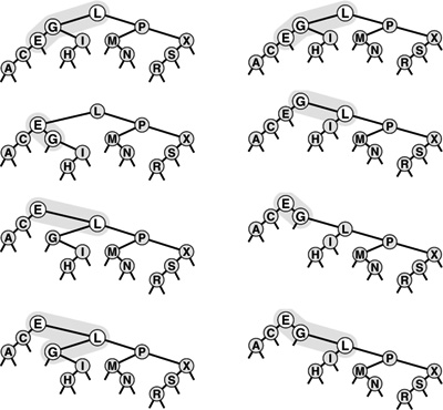
Specifically, as shown in Figure 13.12, every time we encounter a 2-node connected to a 4-node, we transform the pair into a 3-node connected to two 2-nodes, and every time we encounter a 3-node connected to a 4-node, we transform the pair into a 4-node connected to two 2-nodes. Splitting 4-nodes is possible because of the way not only the keys but also the links can be moved around. Two 2-nodes have the same number (four) of links as a 4-node, so we can execute the split without having to propagate any changes below (or above) the split node. A 3-node is not changed to a 4-node just by the addition of another key; another pointer is needed also (in this case, the extra link provided by the split). The crucial point is that these transformations are purely local: No part of the tree needs to be examined or modified other than the part shown in Figure 13.12. Each of the transformations passes up one of the keys from a 4-node to that node’s parent in the tree, and restructures links accordingly.
On our way down the tree, we do not need to worry explicitly about the parent of the current node being a 4-node, because our transformations ensure that, as we pass through each node in the tree, we come out on a node that is not a 4-node. In particular, when we reach the bottom of the tree, we are not on a 4-node, and we can insert the new node directly by transforming either a 2-node to a 3-node or a 3-node to a 4-node. We can think of the insertion as a split of an imaginary 4-node at the bottom that passes up the new key.
One final detail: Whenever the root of the tree becomes a 4-node, we just split it into a triangle of three 2-nodes, as we did for our first node split in the preceding example. Splitting the root after an insertion is slightly more convenient than is the alternative of waiting until the next insertion to do the split because we never need to worry about the parent of the root. Splitting the root (and only this operation) makes the tree grow one level higher.
Figure 13.12 Splitting 4-nodes in a 2-3-4 tree In a 2-3-4 tree, we can split any 4-node that is not the child of a 4-node into two 2-nodes, passing its middle record up to its parent. A 2-node attached to a 4-node (top left) becomes a 3-node attached to two 2-nodes (top right), and a 3-node attached to a 4-node (bottom left) becomes a 4-node attached to two 2-nodes (bottom right).
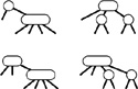
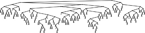
Figure 13.13 depicts the construction of a 2-3-4 tree for a sample set of keys. Unlike standard BSTs, which grow down from the top, these trees grow up from the bottom. Because the 4-nodes are split on the way from the top down, the trees are called top-down 2-3-4 trees. The algorithm is significant because it produces search trees that are nearly perfectly balanced, yet it makes only a few local transformations as it walks through the tree.
Property 13.6 Searches in N-node 2-3-4 trees visit at most lg N + 1 nodes.
Every external node is the same distance from the root: The transformations that we perform have no effect on the distance from any node to the root, except when we split the root (in this case the distance from all nodes to the root is increased by 1). If all the nodes are 2-nodes, the stated result holds, since the tree is like a full binary tree; if there are 3-nodes and 4-nodes, the height can only be lower. ![]()
Property 13.7 Insertions into N-node 2-3-4 trees require fewer than lg N + 1 node splits in the worst case, and seem to require less than one node split on the average.
The worst that can happen is that all the nodes on the path to the insertion point are 4-nodes, all of which will be split. But in a tree built from a random permutation of N elements, not only is this worst case unlikely to occur, but also few splits seem to be required on the average, because there are not many 4-nodes in the trees. For example, in the large tree depicted in Figure 13.14, all but two of the 4-nodes are on the bottom level. Precise analytic results on the average-case performance of 2-3-4 trees have so far eluded the experts, but it is clear from empirical studies that very few splits are used to balance the trees. The worst case is only lg N, and that is not approached in practical situations. ![]()
Figure 13.13 2-3-4 search tree construction This sequence depicts the result of inserting items with keys A S E R C H I N G X into an initially empty 2-3-4 tree. We split each 4-node that we encounter on the search path, thus ensuring that there is room for the new item at the bottom.
The preceding description is sufficient to define an algorithm for searching using 2-3-4 trees that has guaranteed good worst-case performance. However, we are only half of the way to an implementation. Although it would be possible to write algorithms which actually perform transformations on distinct data types representing 2-, 3-, and 4-nodes, most of the tasks that are involved are inconvenient to implement in this direct representation. As in splay BSTs, the overhead incurred in manipulating the more complex node structures could make the algorithms slower than standard BST search. The primary purpose of balancing is to provide insurance against a bad worst case, but we would prefer the overhead cost for that insurance to be low and we also would prefer to avoid paying the cost on every run of the algorithm. Fortunately, as we will see in Section 13.4, there is a relatively simple representation of 2-, 3-, and 4-nodes that allows the transformations to be done in a uniform way with little overhead beyond the costs incurred by standard binary-tree search.
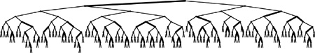
Figure 13.14 A large 2-3-4 tree This 2-3-4 tree is the result of 200 random insertions into an initially empty tree. All search paths in the trees have six or fewer nodes.
![]()
The algorithm that we have described is just one possible way to maintain balance in 2-3-4 search trees. Several other methods that achieve the same goals have been developed.
For example, we can balance from the bottom up. First, we do a search in the tree to find the bottom node where the item to be inserted belongs. If that node is a 2-node or a 3-node, we grow it to a 3-node or a 4-node, just as before. If it is a 4-node, we split it as before (inserting the new item into one of the resulting 2-nodes at the bottom), and insert the middle item into the parent, if the parent is a 2-node or a 3-node. If the parent is a 4-node, we split that node (inserting the middle node from the bottom into the appropriate 2-node), and insert the middle item into its parent, if the parent is a 2-node or a 3-node. If the grandparent is also a 4-node, we continue up the tree in the same way, splitting 4-nodes until we encounter a 2-node or a 3-node on the search path.
We can do this kind of bottom-up balancing in trees that have only 2- or 3-nodes (no 4-nodes). This approach leads to more node splitting during the execution of the algorithm, but is easier to code because there are fewer cases to consider. In another approach, we seek to reduce the amount of node splitting by looking for siblings that are not 4-nodes when we are ready to split a 4-node.
Implementations of all these methods involve the same basic recursive scheme, as we shall see in Section 13.4. We shall also discuss generalizations, in Chapter 16. The primary advantage of the top-down insertion approach that we are considering over other methods is that it can achieve the necessary balancing in one top-down pass through the tree.
Exercises
![]() 13.39 Draw the balanced 2-3-4 search tree that results when you insert items with the keys E A S Y Q U T I O N in that order into an initially empty tree, using the top-down insertion method.
13.39 Draw the balanced 2-3-4 search tree that results when you insert items with the keys E A S Y Q U T I O N in that order into an initially empty tree, using the top-down insertion method.
![]() 13.40 Draw the balanced 2-3-4 search tree that results when you insert items with the keys E A S Y Q U T I O N in that order into an initially empty tree, using the bottom-up insertion method.
13.40 Draw the balanced 2-3-4 search tree that results when you insert items with the keys E A S Y Q U T I O N in that order into an initially empty tree, using the bottom-up insertion method.
![]() 13.41 What are the minimum and maximum heights possible for balanced 2-3-4 trees with
13.41 What are the minimum and maximum heights possible for balanced 2-3-4 trees with N nodes?
![]() 13.42 What are the minimum and maximum heights possible for balanced 2-3-4 BSTs with
13.42 What are the minimum and maximum heights possible for balanced 2-3-4 BSTs with N keys?
![]() 13.43 Draw all the structurally different balanced 2-3-4 BSTs with
13.43 Draw all the structurally different balanced 2-3-4 BSTs with N keys for 2 ≤ N ≤ 12.
![]() 13.44 Find the probability that each of the trees in Exercise 13.43 is the result of the insertion of
13.44 Find the probability that each of the trees in Exercise 13.43 is the result of the insertion of N random distinct elements into an initially empty tree.
13.45 Make a table showing the number of trees for each N from Exercise 13.43 that are isomorphic, in the sense that they can be transformed to one another by exchanges of subtrees in nodes.
![]() 13.46 Describe algorithms for search and insertion in balanced 2-3-4-5-6 search trees.
13.46 Describe algorithms for search and insertion in balanced 2-3-4-5-6 search trees.
![]() 13.47 Draw the unbalanced 2-3-4 search tree that results when you insert items with the keys E A S Y Q U T I O N in that order into an initially empty tree, using the following method. If the search ends in a 2-node or a 3-node, change it to a 3-node or a 4-node, as in the balanced algorithm; if the search ends in a 4-node, replace the appropriate link in that 4-node with a new 2-node.
13.47 Draw the unbalanced 2-3-4 search tree that results when you insert items with the keys E A S Y Q U T I O N in that order into an initially empty tree, using the following method. If the search ends in a 2-node or a 3-node, change it to a 3-node or a 4-node, as in the balanced algorithm; if the search ends in a 4-node, replace the appropriate link in that 4-node with a new 2-node.
13.4 Red–Black Trees
The top-down 2-3-4 insertion algorithm described in the previous section is easy to understand, but implementing it directly is cumbersome because of all the different cases that can arise. We need to maintain three different types of nodes, to compare search keys against each of the keys in the nodes, to copy links and other information from one type of node to another, to create and destroy nodes, and so forth. In this section, we examine a simple abstract representation of 2-3-4 trees that leads us to a natural implementation of the symbol-table algorithms with near-optimal worst-case performance guarantees.
Figure 13.15 3-nodes and 4-nodes in red-black trees The use of two types of links provides us with an efficient way to represent 3-nodes and 4-nodes in 2-3-4 trees. We use red links (thick lines in our diagrams) for internal connections in nodes, and black links (thin lines in our diagrams) for 2-3-4 tree links. A 4-node (top left) is represented by a balanced subtree of three 2-nodes connected by red links (top right). Both have three keys and four black links. A 3-node (bottom left) is represented by one 2-node connected to another (either on the right or the left) with a single red link (bottom right). All have two keys and three black links.
The basic idea is to represent 2-3-4 trees as standard BSTs (2-nodes only), but to add one extra bit of information per node to encode 3-nodes and 4-nodes. We think of the links as being of two different types: red links, which bind together small binary trees comprising 3-nodes and 4-nodes, and black links, which bind together the 2-3-4 tree. Specifically, as illustrated in Figure 13.15, we represent 4-nodes as three 2-nodes connected by red links, and 3-nodes as two 2-nodes connected by a single red link. The red link in a 3-node may be a left link or a right link, so there are two ways to represent each 3-node.
In any tree, each node is pointed to by one link, so coloring the links is equivalent to coloring the nodes. Accordingly, we use one extra bit per node to store the color of the link pointing to that node. We refer to 2-3-4 trees represented in this way as red–black BSTs. The orientation of each 3-node is determined by the dynamics of the algorithm that we shall describe. It would be possible to enforce a rule that 3-nodes all slant the same way, but there is no reason to do so. Figure 13.16 shows an example of a red–black tree. If we eliminate the red links and collapse together the nodes they connect, the result is the 2-3-4 tree in Figure 13.10.
Red–black trees have two essential properties: (i) the standard search method for BSTs works without modification; and (ii) they correspond directly to 2-3-4 trees, so we can implement the balanced 2-3-4 tree algorithm by maintaining the correspondence. We get the best of both worlds: the simple search method from the standard BST, and the simple insertion–balancing method from the 2-3-4 search tree.
The search method never examines the field that represents node color, so the balancing mechanism adds no overhead to the time taken by the fundamental search procedure. Since each key is inserted just once, but may be searched for many times in a typical application, the end result is that we get improved search times (because the trees are balanced) at relatively little cost (because no work for balancing is done during the searches). Moreover, the overhead for insertion is small: we have to take action for balancing only when we see 4-nodes, and there are not many 4-nodes in the tree because we are always breaking them up. The inner loop of the insert procedure is the code that walks down the tree (the same as for the search or search-and-insert operations in standard BSTs), with one extra test added: If a node has two red children, it is a part of a 4-node. This low overhead is a primary reason for the efficiency of red–black BSTs.
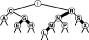
Figure 13.16 A red–black tree This figure depicts a red–black tree that contains the keys A S R C H I N G E X M P L. We can find a key in such a tree with standard BST search. Any path from the root to an external node in this tree has three black links. If we collapse the nodes connected by red links in this tree, we get the 2-3-4 tree of Figure 13.10.
Now, let us consider the red–black representation for the two transformations that we might need to perform when we do encounter a 4-node: If we have a 2-node connected to a 4-node, then we should convert the pair into a 3-node connected to two 2-nodes; if we have a 3-node connected to a 4-node, then we should convert the pair into a 4-node connected to two 2-nodes. When a new node is added at the bottom, we imagine it to be a 4-node that has to be split and its middle node passed up to be inserted into the bottom node where the search ends, which is guaranteed by the top-down process to be either a 2-node or a 3-node. The transformation required when we encounter a 2-node connected to a 4-node is easy, and the same transformation works if we have a 3-node connected to a 4-node in the “right” way, as shown in the first two cases in Figure 13.17.
Figure 13.17 Splitting 4-nodes in a red–black tree In a red–black tree, we implement the operation of splitting a 4-node that is not the child of a 4-node by changing the node colors in the three nodes comprising the 4-node, then possibly doing one or two rotations. If the parent is a 2-node (top), or a 3-node that has a convenient orientation (second from top), no rotations are needed. If the 4-node is on the center link of the 3-node (bottom), a double rotation is needed; otherwise, a single rotation suffices (third from top).
We are left with the two other situations that can arise if we encounter a 3-node connected to a 4-node, as shown in the second two cases in Figure 13.17. (There are actually four situations, because the mirror images of these two can also occur for 3-nodes of the other orientation.) In these cases, the naive 4-node split leaves two red links in a row—the tree that results does not represent a 2-3-4 tree in accordance with our conventions. The situation is not too bad, because we do have three nodes connected by red links: all we need to do is to transform the tree such that the red links point down from the same node.
Fortunately, the rotation operations that we have been using are precisely what we need to achieve the desired effect. Let us begin with the easier of the two remaining cases: the third case in Figure 13.17, where a 4-node attached to a 3-node has split, leaving two red links in a row that are oriented the same way. This situation would not have arisen if the 3-node had been oriented the other way: Accordingly, we restructure the tree to switch the orientation of the 3-node, and thus reduce this case to be the same as the second case, where the naive 4-node split was sufficient. Restructuring the tree to reorient a 3-node is a single rotation with the additional requirement that the colors of the two nodes have to be switched.
Finally, to handle the case where a 4-node attached to a 3-node has split leaving two red links in a row that are oriented differently, we rotate to reduce immediately to the case where the links are oriented the same way, which we then handle as before. This transformation amounts to the same operations as the left-right and right-left double rotations that we used for splay BSTs in Section 13.2, although we have to do slightly more work to maintain the colors properly. Figures 13.18 and 13.19 depict examples of red–black insertion operations.
Program 13.6 is an implementation of insert for red–black trees that performs the transformations that are summarized in Figure 13.17. The recursive implementation makes it possible to perform the color flips for 4-nodes on the way down the tree (before the recursive calls), then to perform rotations on the way up the tree (after the recursive calls). This program would be difficult to understand without the two layers of abstraction that we have developed to implement it. We can check that the recursive trickery implements the rotations depicted in Figure 13.17; then, we can check that the program implements our high-level algorithm on 2-3-4 trees—break up 4-nodes on the way down the tree, then insert the new item into the 2- or 3-node where the search path ends at the bottom of the tree.
Figure 13.18 Insertion into a red–black tree This figure depicts the result (bottom) of inserting a record with key I into the sample red–black tree at the top. In this case, the insertion process consists of splitting the 4-node at C with a color flip (center), then adding the new node at the bottom, converting the node containing H from a 2-node to a 3-node.

Figure 13.20 (which we can think of as a more detailed version of Figure 13.13) shows how Program 13.6 constructs the red–black trees that represent balanced 2-3-4 trees as a sample set of keys is inserted. Figure 13.21 shows a tree built from the larger example that we have been using; the average number of nodes visited during a search for a random key in this tree is just 5.81, as compared to 7.00 for the tree built from the same keys in Chapter 12, and to 5.74, the best possible for a perfectly balanced tree. At a cost of only a few rotations, we get a tree that has far better balance than any of the others that we have seen in this chapter for the same keys.Program 13.6 is an efficient, relatively compact algorithm for insertion using a binary tree structure that is guaranteed to take a logarithmic number of steps for all searches and insertions. It is one of the few symbol-table implementations with that property, and its use is justified in a library implementation where properties of the key sequence to be processed cannot be characterized accurately.
Property 13.8 A search in a red–black tree with N nodes requires fewer than 2 lg N + 2 comparisons.
Only splits that correspond to a 3-node connected to a 4-node in a 2-3-4 tree require a rotation in the red–black tree, so this property follows from Property 13.2. The worst case is when the path to the insertion point consists of alternating 3- and 4-nodes. ![]()
Moreover,Program 13.6 incurs little overhead for balancing, and the trees that it produces are nearly optimal, so it is also attractive to consider as a fast general-purpose searching method.
Property 13.9 A search in a red–black tree with N nodes built from random keys uses about 1.002 lg N comparisons, on the average.
The constant 1.002, which has been confirmed through partial analyses and simulations (see reference section) is sufficiently low that we can regard red–black trees as optimal for practical purposes, but the question of whether red–black trees are truly asymptotically optimal is still open. Is the constant equal to 1? ![]()
Because the recursive implementation in Program 13.6 does some work before the recursive calls and some work after the recursive calls, it makes some modifications to the tree on the way down the search path and some modifications to the tree on the way back up. Therefore, it does not have the property that the balancing is accomplished in one top-down pass. This fact is of little consequence for most applications because the depth of the recursion is guaranteed to be low. For some applications that involve multiple independent processes with access to the same tree, we might need a nonrecursive implementation that actively operates on only a constant number of nodes at any given time (see Exercise 13.66).
Figure 13.19 Insertion into a red–black tree, with rotations This figure depicts the result (bottom) of inserting a record with key G into the red–black tree at the top. In this case, the insertion process consists of splitting the 4-node at I with a color flip (second from top), then adding the new node at the bottom (third from top), then (returning to each node on the search path in the code after the recursive function calls) doing a left rotation at C and a right rotation at R to finish the process of splitting the 4-node.
For an application that carries other information in the trees, the rotation operation might be an expensive one, perhaps causing us to update information in all the nodes in the subtrees involved in the rotation. For such an application, we can ensure that each insertion involves at most one rotation by using red–black trees to implement the bottom-up 2-3-4 search trees that are described at the end of Section 13.3. An insertion in those trees involves splitting 4-nodes along the search path, which involves color changes but no rotations in the red–black representation, followed by one single or double rotation (one of the cases in Figure 13.17) when the first 2-node or a 3-node is encountered on the way up the search path (see Exercise 13.59).
If duplicate keys are to be maintained in the tree, then, as we did with splay BSTs, we must allow items with keys equal to a given node to fall on both sides of that node. Otherwise, severe imbalance could result from long strings of duplicate keys. Again, this observation tells us that finding all items with a given key requires specialized code.
As mentioned at the end of Section 13.3, red–black representations of 2-3-4 trees are among several similar strategies that have been proposed for implementing balanced binary trees (see reference section). As we saw, it is the rotate operations that balance the trees: We have been looking at a particular view of the trees that makes it easy to decide when to rotate. Other views of the trees lead to other algorithms, a few of which we shall mention briefly here.
The oldest and most well-known data structure for balanced trees is the height-balanced, or AVL, tree, discovered in 1962 by Adel’son-Vel’skii and Landis. These trees have the property that the heights of the two subtrees of each node differ by at most 1. If an insertion causes one of the subtrees of some node to grow in height by 1, then the balance condition might be violated. However, one single or double rotation will bring the node back into balance in every case. The algorithm that is based on this observation is similar to the method of balancing 2-3-4 trees from the bottom up: Do a recursive search for the node, then, after the recursive call, check for imbalance and do a single or double rotation to correct it if necessary (see Exercise 13.61). The decision about which rotations (if any) to perform requires that we know whether each node has a height that is 1 less than, the same as, or 1 greater than the height of its sibling. Two bits per node are needed to encode this information in a straightforward way, although it is possible to get by without using any extra storage, using the red–black abstraction (see Exercises 13.62 and 13.65).
Figure 13.20 Construction of a red–black tree This sequence depicts the result of inserting records with keys A S E R C H I N G X into an initially empty red–black tree.
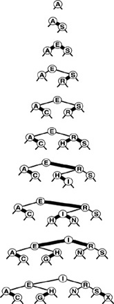
Figure 13.21 A large red–black BST This red–black BST is the result of inserting 200 randomly ordered keys into an initially empty tree. All search misses in the tree use between six and 12 comparisons.
Because 4-nodes play no special role in the bottom-up 2-3-4 algorithm, it is possible to build balanced trees in essentially the same way, but using only 2-nodes and 3-nodes. Trees built in this way are called 2-3 trees, and were discovered by Hopcroft in 1970. There is not enough flexibility in 2-3 trees to give a convenient top-down insertion algorithm. Again, the red–black framework can simplify the implementation, but bottom-up 2-3 trees offer no particular advantage over bottom-up 2-3-4 trees, because single and double rotations are still needed to maintain balance. Bottom-up 2-3-4 trees have slightly better balance and have the advantage of using at most one rotation per insertion.
In Chapter 16, we shall study another important type of balanced tree, an extension of 2-3-4 trees called B-trees. B-trees allow up to M keys per node for large M, and are widely used for search applications that involve huge files.
We have defined red–black trees by correspondence to 2-3-4 trees. It is also amusing to formulate direct structural definitions.
Definition 13.3 A red–black BST is a binary search tree in which each node is marked to be either red or black, with the additional restriction that no two red nodes appear consecutively on any path from an external link to the root.
Definition 13.4 A balanced red–black BST is a red–black BST in which all paths from external links to the root have the same number of black nodes.
Now, an alternative approach to developing a balanced tree algorithm is to ignore the 2-3-4 tree abstraction entirely and formulate an insertion algorithm that preserves the defining property of balanced red–black BSTs through rotations. For example, using the bottom-up algorithm corresponds to attaching the new node at the bottom of the search path with a red link, then proceeding up the search path, doing rotations or color changes, as per the cases in Figure 13.17, to break up any pair of consecutive red links encountered on the path. The fundamental operations that we perform are the same as in Program 13.6 and its bottom-up counterpart, but subtle differences arise, because 3-nodes can orient either way, operations can be performed in different orders, and various different rotation decisions can be used successfully.
Let us summarize: Using red–black trees to implement balanced 2-3-4 trees, we can develop a symbol table where a search operation for a key in a file of, say, 1 million items can be completed by comparing that key with about 20 other keys. In the worst case, no more than 40 comparisons are needed. Furthermore, little overhead is associated with each comparison, so a fast search is ensured, even in a huge file.
Exercises
![]() 13.48 Draw the red–black BST that results when you insert items with the keys E A S Y Q U T I O N in that order into an initially empty tree, using the top-down insertion method.
13.48 Draw the red–black BST that results when you insert items with the keys E A S Y Q U T I O N in that order into an initially empty tree, using the top-down insertion method.
![]() 13.49 Draw the red–black BST that results when you insert items with the keys E A S Y Q U T I O N in that order into an initially empty tree, using the bottom-up insertion method.
13.49 Draw the red–black BST that results when you insert items with the keys E A S Y Q U T I O N in that order into an initially empty tree, using the bottom-up insertion method.
![]() 13.50 Draw the red–black tree that results when you insert letters A through K in order into an initially empty tree, then describe what happens in general when trees are built by insertion of keys in ascending order.
13.50 Draw the red–black tree that results when you insert letters A through K in order into an initially empty tree, then describe what happens in general when trees are built by insertion of keys in ascending order.
13.51 Give a sequence of insertions that will construct the red–black tree shown in Figure 13.16.
13.52 Generate two random 32-node red–black trees. Draw them (either by hand or with a program). Compare them with the (unbalanced) BSTs built with the same keys.
13.53 How many different red–black trees correspond to a 2-3-4 tree that has t 3-nodes?
![]() 13.54 Draw all the structurally different red–black search trees with
13.54 Draw all the structurally different red–black search trees with N keys for 2 ≤ N ≤ 12.
![]() 13.55 Find the probabilities that each of the trees in Exercise 13.43 is the result of inserting
13.55 Find the probabilities that each of the trees in Exercise 13.43 is the result of inserting N random distinct elements into an initially empty tree.
13.56 Make a table showing the number of trees for each N from Exercise 13.54 that are isomorphic, in the sense that they can be transformed to one another by exchanges of subtrees in nodes.
![]()
![]() 13.57 Show that, in the worst case, almost all the paths from the root to an external node in a red–black tree of
13.57 Show that, in the worst case, almost all the paths from the root to an external node in a red–black tree of N nodes are of length 2 lg N.
13.58 How many rotations are required for an insertion into a red–black tree of N nodes, in the worst case?
![]() 13.59 Implement construct, search, and insert for symbol tables with bottom-up balanced 2-3-4 trees as the underlying data structure, using the red–black representation and the same recursive approach as Program 13.6. Hint: Your code can be similar to Program 13.6, but should perform the operations in a different order.
13.59 Implement construct, search, and insert for symbol tables with bottom-up balanced 2-3-4 trees as the underlying data structure, using the red–black representation and the same recursive approach as Program 13.6. Hint: Your code can be similar to Program 13.6, but should perform the operations in a different order.
13.60 Implement construct, search, and insert for symbol tables with bottom-up balanced 2-3 trees as the underlying data structure, using the red–black representation and the same recursive approach as Program 13.6.
13.61 Implement construct, search, and insert for symbol tables with height-balanced (AVL) trees as the underlying data structure, using the same recursive approach as Program 13.6.
![]() 13.62 Modify your implementation from Exercise 13.61 to use red–black trees (1 bit per node) to encode the balance information.
13.62 Modify your implementation from Exercise 13.61 to use red–black trees (1 bit per node) to encode the balance information.
![]() 13.63 Implement balanced 2-3-4 trees using a red–black tree representation in which 3-nodes always lean to the right. Note: This change allows you to remove one of the bit tests from the inner loop for insert.
13.63 Implement balanced 2-3-4 trees using a red–black tree representation in which 3-nodes always lean to the right. Note: This change allows you to remove one of the bit tests from the inner loop for insert.
![]() 13.64Program 13.6 does rotations to keep 4-nodes balanced. Develop an implementation for balanced 2-3-4 trees using a red–black tree representation where 4-nodes can be represented as any three nodes connected by two red links (perfectly balanced or not).
13.64Program 13.6 does rotations to keep 4-nodes balanced. Develop an implementation for balanced 2-3-4 trees using a red–black tree representation where 4-nodes can be represented as any three nodes connected by two red links (perfectly balanced or not).
![]() 13.65 Implement construct, search, and insert for red–black trees without using any extra storage for the color bit, based on the following trick. To color a node red, swap its two links. Then, to test whether a node is red, test whether its left child is larger than its right child. You have to modify the comparisons to accommodate the possible pointer swap, and this trick replaces bit comparisons with key comparisons that are presumably more expensive, but it shows that the bit in the nodes can be eliminated, if necessary.
13.65 Implement construct, search, and insert for red–black trees without using any extra storage for the color bit, based on the following trick. To color a node red, swap its two links. Then, to test whether a node is red, test whether its left child is larger than its right child. You have to modify the comparisons to accommodate the possible pointer swap, and this trick replaces bit comparisons with key comparisons that are presumably more expensive, but it shows that the bit in the nodes can be eliminated, if necessary.
![]() 13.66 Implement a nonrecursive red–black BST insert function (see Program 13.6) that corresponds to balanced 2-3-4 tree insertion with one top-down pass. Hint: Maintain links
13.66 Implement a nonrecursive red–black BST insert function (see Program 13.6) that corresponds to balanced 2-3-4 tree insertion with one top-down pass. Hint: Maintain links gg, g, and p that point, respectively, to the current node’s great-grandparent, grandparent, and parent in the tree. All these links might be needed for double rotation.
13.67 Write a program that computes the percentage of black nodes in a given red–black BST. Test your program by inserting N random keys into an initially empty tree, for N = 103, 104, 105, and 106.
13.68 Write a program that computes the percentage of items that are in 3-nodes and 4-nodes in a given 2-3-4 search tree. Test your program by inserting N random keys into an initially empty tree, for N = 103, 104, 105, and 106.
Figure 13.22 A two-level linked list Every third node in this list has a second link, so we can skip through the list at nearly three times the speed that we could go by following the first links. For example, we can get to the twelfth node in the list, the P, from the beginning by following just five links: second links to C, G, L, N, and then through N’s first link, P.
![]()
![]() 13.69 With 1 bit per node for color, we can represent 2-, 3-, and 4-nodes. How many bits per node would we need to represent 5-, 6-, 7-, and 8-nodes with a binary tree?
13.69 With 1 bit per node for color, we can represent 2-, 3-, and 4-nodes. How many bits per node would we need to represent 5-, 6-, 7-, and 8-nodes with a binary tree?
13.70 Run empirical studies to compute the average and standard deviation of the number of comparisons used for search hits and for search misses in a red–black tree built by insertion of N random keys into an initially empty tree, for N = 103, 104, 105, and 106.
13.71 Instrument your program for Exercise 13.70 to compute the number of rotations and node splits that are used to build the trees. Discuss the results.
13.72 Use your driver program from Exercise 12.30 to compare the self-organizing–search aspect of splay BSTs with the worst-case guarantees of red–black BSTs and with standard BSTs for the search query distributions defined in Exercises 12.31 and 12.32 (see Exercise 13.29).
![]() 13.73 Implement a search function for red–black trees that performs rotations and changes node colors on the way down the tree to ensure that the node at the bottom of the search path is not a 2-node.
13.73 Implement a search function for red–black trees that performs rotations and changes node colors on the way down the tree to ensure that the node at the bottom of the search path is not a 2-node.
![]() 13.74 Use your solution to Exercise 13.73 to implement a remove function for red–black trees. Find the node to be deleted, continue the search to a 3-node or 4-node at the bottom of the path, and move the successor from the bottom to replace the deleted node.
13.74 Use your solution to Exercise 13.73 to implement a remove function for red–black trees. Find the node to be deleted, continue the search to a 3-node or 4-node at the bottom of the path, and move the successor from the bottom to replace the deleted node.
13.5 Skip Lists
In this section, we consider an approach to developing fast implementations of symbol-table operations that seems at first to be completely different from the tree-based methods that we have been considering, but actually is closely related to them. It is based on a randomized data structure and is almost certain to provide near-optimal performance for all the basic operations for the symbol-table ADT that we have been considering. The underlying data structure, which was developed by Pugh in 1990 (see reference section), is called a skip list. It uses extra links in the nodes of a linked list to skip through large portions of a list at a time during a search.
Figure 13.22 gives a simple example, where every third node in an ordered linked list contains an extra link that allows us to skip three nodes in the list. We can use the extra links to speed up search: We scan through the top list until we find the key or a node with a smaller key with a link to a node with a larger key, then use the links at the bottom to check the two intervening nodes. This method speeds up search by a factor of 3, because we examine only about k/3 nodes in a successful search for the kth node on the list.
Figure 13.23 Search and insertion in a skip list By adding more levels to the structure in Figure 13.22 and allowing links to skip variable numbers of nodes, we get an example of a general skip list. To search for a key in the list, we start at the highest level, moving down each time that we encounter a key that is not smaller than the search key. Here (top), we find L by starting at level 3, moving across the first link, then down at G (treating the null link as a link to a sentinel), then across to I, then down to level 2 because S is greater than L, then down to level 1 because M is greater than L. To insert a node L with three links, we link it into the three lists at precisely the places where we found links to greater keys during the search.
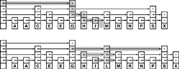
We can iterate this construction, and provide a second extra link to be able to scan faster through the nodes with extra links, and so forth. Also, we can generalize the construction by skipping a variable number of nodes with each link.
Definition 13.5 A skip list is an ordered linked list where each node contains a variable number of links, with the ith links in the nodes implementing singly linked lists that skip the nodes with fewer than i links.
Figure 13.23 depicts a sample skip list, and shows an example of searching and inserting a new node. To search, we scan through the top list until we find the search key or a node with a smaller key that has a link to a node with a larger key; then, we move to the second-from-top list and iterate the procedure, continuing until the search key is found or a search miss happens on the bottom level. To insert, we search, linking in the new node when moving from level k to level k–1 if the new node has at least k extra links.
The internal representation of the nodes is straightforward. We replace the single link in a singly linked list by an array of links, and an integer that contains the number of links in the node. Memory management is perhaps the most complicated aspect of skip lists—we will examine the type declarations and the code for allocating new nodes shortly, when we consider insertion. For the moment, it suffices to note that we can access the node that follows node t on the (k + 1)st level in the skip list by accessing t->next[k]. The recursive implementation in Program 13.7 shows that searching in skip lists not only is a straightforward generalization of searching in singly linked lists, but also is similar to binary search or searching in BSTs. We test whether the current node has the search key. Then, if it does not, we compare the key in the current node with the search key. We do one recursive call if it is larger and a different recursive call if it is smaller.
The first task that we face when we want to insert a new node into a skip list is to determine how many links we want that node to have. All the nodes have at least one link; following the intuition depicted in Figure 13.22, we can skip t nodes at a time on the second level if one out of every t nodes has at least two links; iterating, we come to the conclusion that we want one out of every tj nodes to have at least j + 1 links.
Figure 13.24 Skip-list construction This sequence depicts the result of inserting items with keys A S E R C H I N G into an initially empty skip list. Nodes have j links with probability 1/2j.
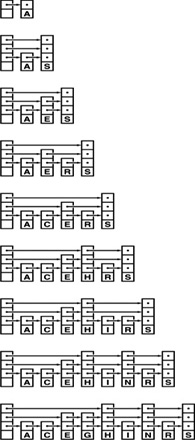
To make nodes with this property, we randomize, using a function that returns j + 1 with probability 1/tj. Given j, we create a new node with j links and insert it into the skip list using the same recursive schema as we did for search, as illustrated in Figure 13.23. After we have reached level j, we link in the new node each time that we move down to the next level. At that point, we have established that the item in the current node is less than the search key and links (on level j) to a node that is not less than the search key.
To initialize a skip list, we build a head node with the maximum number of levels that we will allow in the list, with null pointers at all levels. Programs 13.8 and 13.9 implement initialization and insertion for skip lists.
Figure 13.24 shows the construction of a skip list for a sample set of keys when inserted in random order; Figure 13.25 shows a larger example; and Figure 13.26 shows the construction of a skip list for the same set of keys as in Figure 13.24, but inserted in increasing order. Like those of randomized BSTs, the stochastic properties of skip lists do not depend on the order in which keys are inserted.
Property 13.10 Search and insertion in a randomized skip list with parameter t require about (t logt N)/2 = (t=(2l g t)) lg N comparisons, on the average.
We expect the skip list to have about logt N levels, because logt N is greater than the smallest j for which tj = N. On each level, we expect that about t nodes were skipped on the previous level, and that we should have to go through about half of them, on the average, before dropping to the next level. The number of levels is small, as is clear from the example in Figure 13.25, but the precise analysis that establishes this is not elementary (see reference section).![]()
Figure 13.25 A large skip list This skip list is the result of inserting 50 randomly ordered keys into an initially empty list. We can access any node by following 7 or fewer links.
![]()
Property 13.11 Skip lists have (t/(t –1))N links on the average.
There are N/t links on the bottom, N/t2 links on second level, and so forth, for a total of about
N (1 + 1/t+ 1/t2 + 1/t3…)= N/(1-1/t)
links in the whole list.![]()
Picking an appropriate value of t leads us immediately to a time–space tradeoff. When t = 2, skip lists need about lg N comparisons and 2N links, on the average—performance comparable with the best that we have seen with BSTs. For larger t, the time for search and insert is longer, but the extra space for links is smaller. Differentiating the expression in Property 13.10, we find that the choice t = e minimizes the expected number of comparisons for searching in a skip list. The following table gives the value of the coefficient of N lg N in the number of comparisons needed to construct a table of N items:
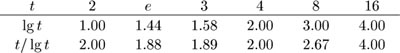
If doing comparisons, following links, and moving down recursively have costs that differ substantially, we can do a more refined calculation along these lines (see Exercise 13.83).
Because the search time is logarithmic, we can reduce the space overhead to not much more than that for singly-linked lists (if space is tight) by increasing t. Precise estimates of running time depend on assessment of the relative costs of following links across the lists and the recursive calls to move down to the next level. We shall revisit this kind of time–space tradeoff again in Chapter 16, when we look at the problem of indexing huge files.
Figure 13.26 Skip-list construction with keys in order This sequence depicts the result of inserting items with keys A C E G H I N R S into an initially empty skip list. Stochastic properties of the list do not depend on the key insertion order.
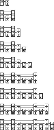
Other symbol-table functions are straightforward to implement with skip lists. For example,Program 13.10 gives an implementation of the remove function, using the same recursive scheme that we used for insert in Program 13.9. To delete, we unlink the node from the lists at each level (where we linked it in for insert), and we free the node after unlinking it from the bottom list (as opposed to creating it before traversing the list for insert). To implement join, we merge the lists (see Exercise 13.78); to implement select, we add a field to each node that gives the number of nodes skipped by the highest-level link to it (see Exercise 13.77).
Although skip lists are easy to conceptualize as a systematic way to move quickly through a linked list, it is also important to understand that the underlying data structure is nothing more than an alternative representation of a balanced tree. For example, Figure 13.27 shows the skip-list representation of the balanced 2-3-4 tree in Figure 13.10. We can implement the balanced 2-3-4 tree algorithms of Section 13.3 using the skip-list abstraction, rather than the red–black tree abstraction of Section 13.4. The resulting code is somewhat more complicated than the implementations that we have considered (see Exercise 13.80). We shall revisit this relationship between skip lists and balanced trees in Chapter 16.
Figure 13.27 Skip-list representation of a 2-3-4 tree This skip list is a representation of the 2-3-4 tree in Figure 13.10. In general, skip lists correspond to balanced multiway trees with one or more links per node (1-nodes, with no keys and 1 link, are allowed). To build the skip list corresponding to a tree, we give each node a number of links equal to its height in the tree, and then link the nodes horizontally. To build the tree corresponding to a skip list, we group skipped nodes, and recursively link them to nodes at the next level.
![]()
The ideal skip list illustrated in Figure 13.22 is a rigid structure that is as difficult to maintain, when we insert a new node, as is the ordered array for binary search, because the insertion involves changing all the links in all the nodes after the node inserted. One way to loosen the structure is to build lists where each link skips either one, two, or three links on the level below: this arrangement corresponds to 2-3-4 trees, as illustrated in Figure 13.27. The randomized algorithm discussed in this section is another effective way to loosen the structure; we shall consider other alternatives in Chapter 16.
Exercises
13.75 Draw the skip list that results when you insert items with the keys E A S Y Q U T I O N in that order into an initially empty list, assuming that randX returns the sequence of values 1, 3, 1, 1, 2, 2, 1, 4, 1, and 1.
![]() 13.76 Draw the skip list that results when you insert items with the keys
13.76 Draw the skip list that results when you insert items with the keys A E I N O Q S T U Y in that order into an initially empty list, assuming the same randX return values as for Exercise 13.75.
13.77 Implement the select operation for a skip-list–based symbol table.
• 13.78 Implement the join operation for a skip-list–based symbol table.
![]() 13.79 Modify the implementations of search and insert given in Program 13.7 and Program 13.9 to end lists with a sentinel node, instead of 0.
13.79 Modify the implementations of search and insert given in Program 13.7 and Program 13.9 to end lists with a sentinel node, instead of 0.
![]() 13.80 Use skip lists to implement construct, search, and insert for symbol tables with the balanced 2-3-4 tree abstraction.
13.80 Use skip lists to implement construct, search, and insert for symbol tables with the balanced 2-3-4 tree abstraction.
![]() 13.81 How many random numbers are needed, on the average, to build a skip list with parameter
13.81 How many random numbers are needed, on the average, to build a skip list with parameter t, using the randX() function in Program 13.9?
![]() 13.82 For
13.82 For t = 2, modify Program 13.9 to eliminate the for loop in randX. Hint: The final j bits in the binary representation of a number t assume any particular j-bit value with probability 1/2j.
13.83 Choose the value of t that minimizes the search cost for the case that following a link costs α times as much as doing a comparison and that moving down one level of recursion costs ß times as much as doing a comparison.
![]() 13.84 Develop a skip list implementation that has the pointers themselves in the nodes instead of the pointer to an array of pointers that we used in Programs 13.7 through 13.10. Hint: Put the array at the end of
13.84 Develop a skip list implementation that has the pointers themselves in the nodes instead of the pointer to an array of pointers that we used in Programs 13.7 through 13.10. Hint: Put the array at the end of node.
13.6 Performance Characteristics
How do we choose among randomized BSTs, splay BSTs, red–black BSTs, and skip lists for a particular application? We have concentrated on the differing nature of these algorithms’ performance guarantees. Time and space are always primary considerations, but we must also consider a number of other factors. In this section, we shall briefly discuss implementation issues, empirical studies, estimates of running time, and space requirements.
All the tree-based algorithms depend on rotations; implementation of rotations along the search path is an essential ingredient of most balanced tree algorithms. We have used recursive implementations that implicitly save pointers to nodes on the search path in local variables on the recursion stack, but each of the algorithms can be implemented in a nonrecursive fashion, operating on a constant number of nodes and performing a constant number of link operations per node in one top-down pass through the tree.
Randomized BSTs are the simplest to implement of the three treebased algorithms. The prime requirements are to have confidence in the random-number generator and to avoid spending too much time generating the random bits. Splay BSTs are slightly more complicated, but are a straightforward extension to the standard root insertion algorithm. Red–black BSTs involve slightly more code still, to check and manipulate the color bits. One advantage of red–black trees over the other two is that the color bits can be used for a consistency check for debugging, and for a guarantee of a quick search at any time during the lifetime of the tree. There is no way to know from examining a splay BST whether or not the code that produced it made all the proper transformations; a bug might lead (only!) to performance problems. Similarly, a bug in the random-number generator for randomized BSTs or skip lists could lead to otherwise-unnoticed performance problems.
Skip lists are easy to implement, and are particularly attractive if a full range of symbol-table operations is to be supported, because search, insert, remove, join, select, and sort all have natural implementations that are easy to formulate. The inner loop for searching in skip lists is longer than that for trees (it involves an additional index into the pointer array or an additional recursive call to move down a level), so the time for search and insert is longer. Skip lists also put the programmer at the mercy of the random-number generator—debugging a program whose behavior is random is a challenge, and some programmers find it particularly unsettling to work with nodes having a random number of links.
Table 13.1 gives empirical data on the performance of the four methods that we have discussed in this chapter, and on the elementary BST implementations from Chapter 12, for keys that are random 32-bit integers. The information in this table confirms what we expect from the analytic results in Sections 13.2, 13.4, and 13.5. Red–black BSTs are much faster than the others for random keys. Paths in red–black BSTs are 35 percent shorter than in randomized or splay BSTs, and there is less work to do in the inner loop. Randomized trees and skip lists require that we generate at least one new random number for every insertion, and splay BSTs involve a rotation at every node for every insertion and every search. By contrast, the overhead for red–black BSTs is that we check the value of 2 bits at every node during insertion, and occasionally need to do a rotation. For nonuniform access, splay BSTs may involve shorter paths, but this savings is likely to be offset by the fact that both search and insertion involve rotations at every node in the inner loop, except possibly in extreme cases.
Splay BSTs require no extra space for balance information, red–black BSTs require 1 extra bit, and randomized BSTs require a count field. For many applications, the count field is maintained for other reasons, so it may not represent an extra cost for randomized BSTs. Indeed, we might need to add this field if we use splay BSTs, red–black BSTs or skip lists. If necessary, we can make red–black BSTs as spaceefficient as splay BSTs by eliminating the color bit (see Exercise 13.65). In modern applications, space is less critical than it once was, but the careful programmer still needs to be vigilant against waste. For example, we need to be aware that some systems might use a whole 32-bit word for a small count field or a 1-bit color field in a node, and that some other systems might pack the fields in memory such that unpacking them requires a significant amount of extra time. If space is tight, skip lists with large t can reduce by nearly one-half the space for links, at the cost of a slower—but still logarithmic—search. With some programming, the tree-based methods can also be implemented with one link per node (see Exercise 12.68).
Table 13.1 Empirical study of balanced tree implementations
These relative timings for building and searching BSTs from random sequences of N 32-bit integers, for various values of N, indicate that all the methods have good performance, even for huge tables, but that red–black trees are significantly faster than are the other methods. All the methods use standard BST search, except splay BSTs, where we splay on search to bring frequently accessed keys near the top, and skip lists, which use essentially the same algorithm with a different underlying data structure.
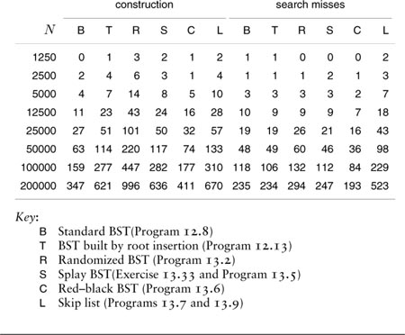
In summary, all the methods that we have discussed in this chapter will provide good performance for typical applications, and each has its virtues for people interested in developing a high-performance symbol-table implementation. Splay BSTs will provide good performance as a self-organizing search method, particularly when frequent access to a small set of keys is a typical pattern; randomized BSTs are likely to be faster and easier to implement for a full-function symbol table BST; skip lists are easy to understand and can provide logarithmic search with less space than the other methods, and red–black BSTs are attractive for symbol-table library implementations, because they provide guaranteed performance bounds in the worst case and the fastest search and insertion algorithms for random data.
Beyond specific uses in applications, this panoply of solutions to the problem of developing efficient implementations of the symboltable ADT is important because it illustrates fundamental approaches to algorithm design that are available to us when we consider solutions to other problems. In our constant quest for simple, optimal algorithms, we often encounter useful near-optimal algorithms, such as the ones discussed here. Moreover, as we saw with sorting, comparisonbased algorithms such as these are only the beginning of the story—by moving to a lower-level abstraction, where we can process pieces of keys, we can develop implementations that are even faster than the ones discussed in this chapter, as we shall see in Chapters 14 and 15.
Exercises
13.85 Develop a symbol-table implementation using randomized BSTs that includes a destructor, a copy constructor, and an overloaded assignment operator, and supports the construct, count, search, insert, remove, join, select, and sort operations for first-class symbol-table ADTs with client item handles (see Exercises 12.6 and 12.7).
13.86 Develop a symbol-table implementation using skip lists that includes a destructor, a copy constructor, and an overloaded assignment operator, and supports the construct, count, search, insert, remove, join, select, and sort operations for first-class symbol-table ADTs with client item handles (see Exercises 12.6 and 12.7).