
2. An Introduction to SQL
Structured Query Language (SQL) is one programming language used to interact with a relational database, and it is the language used in SQLite. The language supports the ability to define database structure, manipulate data, and read the data contained in the database.
Although SQL has been standardized by both the American National Standards Institute (ANSI) and the International Organization for Standardization (ISO), vendors frequently add proprietary extensions to the language to better support their platforms. This chapter primarily focuses on SQL as it is implemented in SQLite, the database system that is included in Android. Most of the concepts in this chapter do apply to SQL in general, but the syntax may not be the same for other database systems.
This chapter covers three areas of SQL:
![]() Data Definition Language (DDL)
Data Definition Language (DDL)
![]() Data Manipulation Language (DML)
Data Manipulation Language (DML)
![]() Queries
Queries
Each area has a different role in a database management system (DBMS) and a different subset of commands and language features.
Data Definition Language
Data Definition Language (DDL) is used to define the structure of a database. This includes the creation, modification, and removal of database objects such as tables, views, triggers, and indexes. The entire collection of DDL statements defines the schema for the database. The schema is what defines the structural representation of the database. The following SQL commands are usually used to build DDL statements:
![]()
CREATE: Creates a new database object
![]()
ALTER: Modifies an existing database object
![]()
DROP: Removes a database object
The following sections describe how the CREATE, ALTER, and DROP commands can be used with different database objects.
Tables
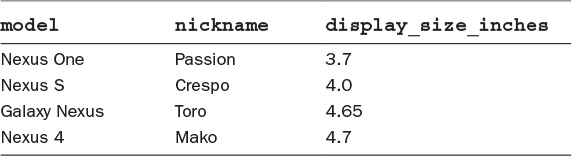
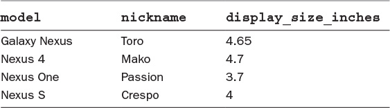
Tables, as discussed in Chapter 1, “Relational Databases,” provide the relations in a relational database. They are what house the data in the database by providing rows representing a data item, and columns representing attributes of each item. Table 2.1 shows an example of a table that contains device information.
SQLite supports the CREATE, ALTER, and DROP commands with regard to tables. These commands allow tables to be created, mutated, and deleted respectively.
CREATE TABLE
The CREATE TABLE statement begins by declaring the name of the table that will be created in the database, as shown in Figure 2.1. Next, the statement defines the columns of the table by providing a column name, data type, and any constraints for the column. Constraints place limits on the values that can be stored in a given attribute of a table.

Listing 2.1 shows a CREATE TABLE statement that creates a table named device with three columns: model, nickname, and display_size_inches.
Listing 2.1 Creating the device Table
CREATE TABLE device (model TEXT NOT NULL,
nickname TEXT,
display_size_inches REAL);
Note
The discussion of SQL data types is deferred to Chapter 3, “An Introduction to SQLite.” For now, it is enough to know that TEXT represents a text string and REAL a floating-point number.
If the SQL statement from Listing 2.1 is run and returns without an error, the device table is created with three columns: model, nickname, and display_size_inches of types TEXT, TEXT, and REAL respectively. In addition, the table has a constraint on the model column to ensure that every row has a non-null model name. The constraint is created by appending NOT NULL to the end of the column name in the CREATE statement. The NOT NULL constraint causes SQLite to throw an error if there is an attempt to insert a row into the table that contains a null value for the model column.
At this point, the table can be used to store and retrieve data. However, as time passes, it is often necessary to make changes to existing tables to support the changing needs of software. This is done with an ALTER TABLE statement.
ALTER TABLE
The ALTER TABLE statement can be used to modify an existing table by either adding new columns or renaming the table. However, the ALTER TABLE statement does have limitations in SQLite. Notice from Figure 2.2 that there is no way to rename or remove a column from a table. This means that once a column is added, it will always be a part of the table. The only way to remove a column is to remove the entire table and re-create the table without the column to be removed. Doing this, however, also removes all the data that was in the table. If the data is needed when the table is re-created, an app must manually copy the data from the old table into the new table.

As an example, the SQL code to add a new column to the device table is shown in Listing 2.2. The new column is named memory_mb and it is of type REAL. It is used to track the amount of memory in a device.
Listing 2.2 Adding a New Row to the device Table
ALTER TABLE device ADD COLUMN memory_mb REAL;
DROP TABLE
The DROP TABLE statement is the simplest table operation; it removes the table from the database along with all the data it contains. Figure 2.3 shows an overview of the DROP TABLE statement. In order to remove a table, the DROP TABLE statement needs only the name of the table to be removed.
The device table can be removed with the statement shown in Listing 2.3.
Listing 2.3 Removing the device Table
DROP TABLE device;
Care should be taken when using the DROP TABLE statement. Once the DROP TABLE statement completes, the data is irrevocably removed from the database.
Indexes
An index is a database object that can be used to speed up queries. To understand what an index is, a discussion of how databases (SQLite in this case) find rows in a table is helpful.
Suppose an app needs to find a device with a specific model from the device table shown in Table 2.1. The application code would run a query against the table, passing the desired model name. Without an index, SQLite would then have to examine every row in the table to find all rows that match the model name. This is referred to as a full table scan as the entire table is being read. As the table grows, a full table scan takes more time as the database needs to inspect an increasing number of rows. It would take significantly more time to perform a full table scan on a table with four million rows than on a table with only four rows.
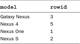
An index can speed up a query by keeping track of column values in an additional table that can be quickly scanned to avoid a full table scan. Table 2.2 shows another version of the device table presented in Table 2.1.

Notice the new column in Table 2.2 called rowid. SQLite automatically creates this column when creating a table unless you specifically direct it not to. While an app will logically consider the device table to look like Table 2.1 (without the rowid), in memory the device table actually looks more like Table 2.2 with the rowid included.
Note
The rowid column can also be accessed using standard SQL queries.
The rowid is a special column in SQLite and can be used to implement indexes. The rowid for each row in a table is guaranteed to be an increasing integer that uniquely identifies the row. However, notice in Table 2.2 that the rowid values may not be consecutive. This is because rowids are generated as rows are inserted to a table, and rowid values are not reused when rows are removed from a table. In Table 2.2, a row with a rowid of 4 was inserted into the table at one point but has since been deleted. Even though rowids may not be consecutive, they remain ordered as rows are added to the table.
Using the rowid, SQLite can quickly perform a lookup on a row since internally it uses a B-tree to store row data with the rowid as the key.
Note
Using the rowid to query a table also prevents the full table scan. However, rowids are usually not convenient to use as they rarely have any other purpose in an app’s business logic.
When an index is created for a table column, SQLite creates a mapping of the row values for that column and the corresponding rowid. Table 2.3 shows such a mapping for the model column of the device table.
Notice that the model names are sorted. This allows SQLite to perform a binary search to find the matching model. Once it is found, SQLite can access the rowid for the model and use that to perform the lookup of the row data in the device table without the need for a full table scan.
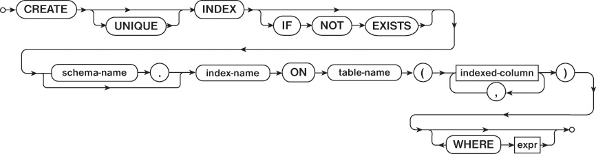
CREATE INDEX
The CREATE INDEX statement needs a name as well as a column definition for the index. In the simplest case, the index has a column definition that includes a single column that is frequently used to search a table during queries. Figure 2.4 shows the structure of the CREATE INDEX statement.
Listing 2.4 shows how to create an index on the model column of the device table.
Listing 2.4 Creating an Index on model
CREATE INDEX idx_device_model ON device(model);
Unlike tables, indexes cannot be modified once they are created. Therefore, the ALTER keyword cannot be applied to indexes. To modify an index, the index must be deleted with a DROP INDEX statement and then re-created with a CREATE INDEX statement.
DROP INDEX
The DROP INDEX statement, as shown in Figure 2.5, has the same form as other DROP statements such as DROP TABLE. It needs only the name of the index to be removed.
Listing 2.5 shows how to drop the index that was created in Listing 2.4.
Listing 2.5 Deleting the Index on model
DROP INDEX idx_device_model;
Views
A view can be thought of as a virtual table in a database. Like a table, it can be queried against to get a result set. However, it does not physically exist in the database in the same way that a table does. Instead, it is the stored result of a query that is run to generate the view. Table 2.4 shows an example of a view.
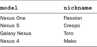
Notice that the view from Table 2.4 contains only a subset of the columns of the device table. Even if more columns are added to the table, the view will remain the same.
Note
SQLite supports only read-only views. This means that views can be queried but do not support the DELETE, INSERT, or UPDATE operations.
CREATE VIEW
The CREATE VIEW statement assigns a name to a view in a similar manner to other CREATE statements (CREATE TABLE, CREATE VIEW, etc.), as shown in Figure 2.6. In addition to a name, the CREATE VIEW statement includes a way to define the content of the view. The view’s content can be defined by a SELECT statement, which returns the columns to be included in the view as well as places limits on which rows should be included in the view.
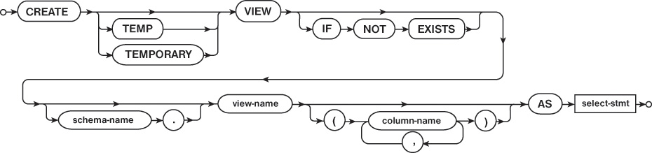
Listing 2.6 shows the SQL code needed to create the view from Table 2.4. The code creates a view named device_name which includes the model and nickname columns from the device table. Because the SELECT statement has no WHERE clause, all rows from the device table are included in the view.
Listing 2.6 Creating the device_name View
CREATE VIEW device_name AS SELECT model, nickname FROM device;
Note
SELECT statements are covered in more detail later in the chapter.
Views in SQLite are read-only and don’t support the DELETE, INSERT, or UPDATE operations. In addition, they cannot be modified with an ALTER statement. As with indexes, in order to modify a view, it must be deleted and re-created.
DROP VIEW
DROP VIEW works like the other DROP commands that have been discussed thus far. It takes the name of the view to be deleted and removes it. The details of the DROP VIEW statement can be seen in Figure 2.7.
Listing 2.7 removes the device_name view that was created in Listing 2.6.
Listing 2.7 Removing the device_name View
DROP VIEW device_name;
Triggers
The final database object that can be manipulated by DDL is a trigger. Triggers provide a way to perform an operation in response to a database event. For example, a trigger can be created to run an SQL statement whenever a row is added or deleted in the database.
CREATE TRIGGER
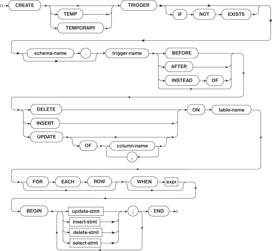
Like other CREATE statements discussed previously, the CREATE TRIGGER statement assigns a name to a trigger by providing the name to the CREATE TRIGGER statement. After the name, an indication of when the trigger needs to run is defined. This definition of when a trigger should run has two parts: the operation that causes the trigger to run, and when the trigger should run in relation to that operation. For example, a trigger can be declared to run before, after, or instead of any DELETE, INSERT, or UPDATE operation. The DELETE, INSERT, and UPDATE operations are part of SQL’s DML, discussed later in the chapter. Figure 2.8 shows an overview of the CREATE TRIGGER statement.
Listing 2.8 shows the creation of a trigger on the device table that sets the insertion time of any newly inserted rows.
Listing 2.8 Creating a Trigger on the device Table
ALTER TABLE device ADD COLUMN insert_date INTEGER;
CREATE TRIGGER insert_date AFTER INSERT ON device
BEGIN
UPDATE device
SET insert_date = datetime('now');
WHERE _ROWID_ = NEW._ROWID_;
END;
Before the insertion date can be tracked, the insert_date column must be added to the device table. This is done with an ALTER TABLE statement prior to the trigger being created (the insert_date column needs to exist before it can be referenced in the trigger definition).
After the ALTER TABLE statement has been run, the device table will contain the values shown in Table 2.5.
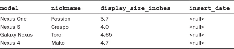
Notice that the value of insert_date is null for all rows. This is because the column was added after the table was created and the ALTER TABLE statement did not specify a default value to add to existing rows.
Now that the trigger is defined, the following INSERT statement can be run to insert a new row in the table:
INSERT INTO device (model, nickname, display_size_inches)
VALUES ("new_model", "new_nickname", 4);
Table 2.6 shows the rows that are now in the device table.
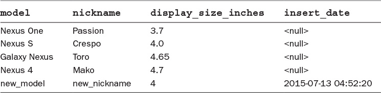
Notice that the new row has a timestamp to indicate when it was added. This column was populated by the insert_date trigger automatically when the INSERT statement was run. Let’s dive a little deeper into the details of the trigger to explore how it works.
The first line of the trigger simply assigns it a name and dictates that it should be run after an INSERT statement on the device table:
CREATE TRIGGER insert_date AFTER INSERT ON device
The actual details of the trigger are between the BEGIN and END statements:
BEGIN
UPDATE device
SET insert_date = datetime('now')
WHERE _ROWID_ = NEW._ROWID_;
END;
The previous statements cause an UPDATE statement to run, setting the insert_date to the current time. The UPDATE statement defines which table to operate on (device) and what values to set (column insert_date to the current date and time). The interesting part of the insert_date trigger is the WHERE clause in the UPDATE statement:
WHERE _ROWID_ = NEW._ROWID_;
Recall from the discussion of indexes that rows in an SQLite database have a rowid that is added by the database automatically and that this rowid column can be accessed. The WHERE clause in the UPDATE statement accesses this rowid column by using NEW._ROWID_. _ROWID_ is the special name of the column that can be used to access the rowid for a given row.
This WHERE clause causes the UPDATE statement to run only when the WHERE clause evaluates to true. In the insert_date trigger, this happens only when the row being manipulated by the trigger is the current row. Failure to include the WHERE clause causes the UPDATE statement to run on every row of the table.
To ensure that the current row matches the row being inserted, the NEW keyword is used. In a trigger, NEW represents the updated column values of the row being updated. In a similar fashion, OLD can be used to access the old values of a row that is being processed.
Triggers cannot be altered. In order for them to be modified, they need to be deleted and re-created.
DROP TRIGGER
The DROP TRIGGER statement works like the other DROP statements introduced in this chapter. As shown in Figure 2.9, it takes the name of the trigger that should be removed and deletes it.
Listing 2.9 removes the insert_date trigger.
Listing 2.9 Removing the DROP TRIGGER Statement
DROP TRIGGER insert_date;
The previous sections provided an overview of the DDL that is supported by SQLite. Using the DDL, it is possible to define database objects that can be used to store data in a local database. The next section discusses ways to manipulate data that can be stored in a database.
Warning
While triggers can be an attractive feature of SQL, it is important to understand that they are not without their faults. Because the database runs a trigger automatically in response to an action performed on the database, a trigger may produce unexpected side effects. It may not always be obvious to application code that a trigger has been added to a table, and that could cause a database operation initiated by the trigger to have unintended results. In a lot of cases, it may be better for the app to move certain logic to the application code rather than add the same functionality in a trigger.
Data Manipulation Language
Data Manipulation Language (DML) is used to read and modify the data in a database. This includes inserting and updating rows in tables. Once the structure of the database has been defined with DDL, DML can be used to alter the data in the table. The main difference between DDL and DML is that DDL is used to define the structure of the data in a database, whereas DML is used to process the data itself.
DML consists of three operations that can be applied to rows in a table:
![]()
INSERT: Adds a row to a table
![]()
DELETE: Removes a row from a table
![]()
UPDATE: Modifies the attribute values for a row in a table
INSERT
The INSERT statement is used to add rows to a table. Specifying what data should be inserted into the table and which columns that data should be inserted into can be done in three ways: using the VALUES keyword, using a SELECT statement, and using the DEFAULT keyword. Figure 2.10 shows an overview of the INSERT statement.
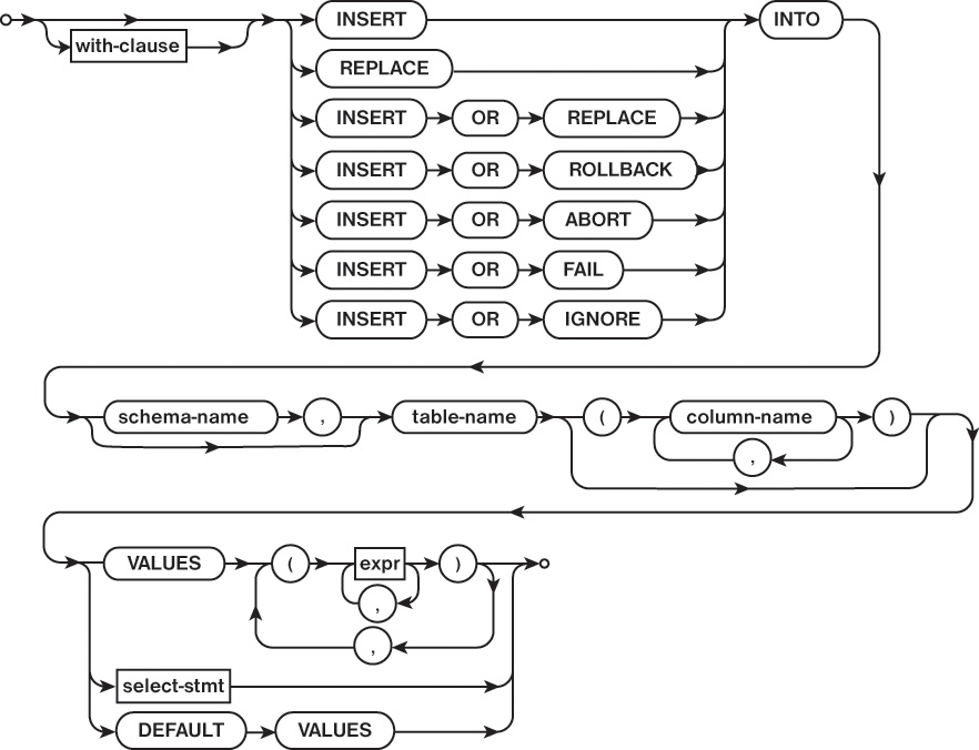
VALUES
When using the VALUES keyword, the INSERT statement must specify the values to be instated for each row. This is done by using two lists in the INSERT statement to specify the destination column and the value for the column. The order must match so that the column name and the value have the same offset in the list.
When using the VALUES keyword with the INSERT statement, only a single row can be inserted into a table per INSERT statement. This means that multiple INSERT statements are needed in order to insert multiple rows into a table.
SELECT
Using the SELECT statement to specify row content in an INSERT statement causes the row that is inserted to contain the result set returned by the SELECT statement. When using this form of the INSERT statement, it is possible to insert multiple rows with one INSERT statement.
DEFAULT
The DEFAULT keyword is used to insert a row into the table that contains only default values for each column. When defining a table, it is possible to assign a default value for each column.
Listing 2.10 shows a basic example of using multiple INSERT statements to populate the data into the device table that was presented in Table 2.1.
Listing 2.10 Populating the Table with Multiple INSERT Statements
INSERT INTO device (model, nickname, display_size_inches)
VALUES ("Nexus One", "Passion", 3.7);
INSERT INTO device (model, nickname, display_size_inches)
VALUES ("Nexus S", "Crespo", 4.0);
INSERT INTO device (model, nickname, display_size_inches)
VALUES ("Galaxy Nexus", "Toro", 4.65);
INSERT INTO device (model, nickname, display_size_inches)
VALUES ("Nexus 4", "Mako", 4.7);
After rows have been inserted into a table, they can be altered using an UPDATE statement.
UPDATE
An UPDATE statement is used to modify data that already exists in a table. Like the INSERT statement, the table name, affected columns, and the new values for the affected columns must be specified. In addition, a WHERE clause may be specified to limit the manipulation to only specific rows. If a WHERE clause is not present in the UPDATE statement, all rows of the table will be manipulated. Figure 2.11 shows an overview of the UPDATE statement.
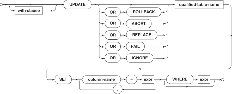
Listing 2.11 shows an example of an UPDATE statement that processes all rows of a table. The UPDATE statement sets the model column to “Nexus” for all rows of the table.
Listing 2.11 Processing All Rows with UPDATE
UPDATE device SET model = "Nexus";
Listing 2.12 makes use of the WHERE clause to update specific rows of the table. The UPDATE statement sets the model name to “Nexus 4” for all rows that have a device_size_inches greater than 4.
Listing 2.12 Using UPDATE with a WHERE Clause
UPDATE device SET model = "Nexus 4" WHERE device_size_inches > 4;
DELETE
The DELETE statement, shown in Figure 2.12, is used to remove rows from a table. Like the UPDATE statement, it can be used with a WHERE clause to remove only specific rows. If the WHERE clause is not used, the DELETE statement removes all rows from a table. The table will still exist in the database; it will just be empty.
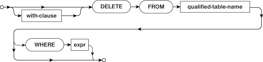
Listing 2.13 shows a DELETE statement that removes all rows from the device table where the display_size_inches is greater than 4.
Listing 2.13 Removing Rows with DELETE
DELETE FROM device WHERE display_size_inches > 4;
Now that DDL and DML have been discussed, it is time to start looking at the parts of SQL that allow queries to be run against a database. This is done with the SELECT statement.
Queries
In addition to defining database structure and manipulating data in a database, SQL provides a way to read the data. In most cases, this is done by querying the database using a SELECT statement. Running database queries is heavily based on the relational algebra and relational calculus concepts that were discussed in Chapter 1.
Figure 2.13 shows the structure for the SELECT statement in SQL.

The SELECT statement can be fairly complicated as can be seen in Figure 2.13. In most cases, it starts with the SELECT keyword and is followed by the projection of the query. Recall from Chapter 1 that the projection is the subset of columns in the table. For the SELECT statement, the projection is the list of columns that should be returned from the table. The projection either can list the desired columns or may use a * to represent all the columns of the table.
After the desired columns have been specified, a SELECT statement must include a FROM clause to indicate where the input data is located. Listing 2.14 contains two queries that return data from the device table. The first query uses the * character to return all columns from the table, and the second query lists a subset of columns to be returned from the device table.
SELECT * FROM device;
SELECT model, nickname FROM device;
The result set returned from each of the queries in Listing 2.14 includes all of the rows of the table. To limit the query to specific rows, the WHERE clause can be added to a SELECT statement.
The WHERE clause describes which rows the query should return. The WHERE clause in a SELECT statement works the same way as a WHERE clause in an UPDATE or DELETE statement. Listing 2.15 shows a SELECT statement that returns all columns for rows that contain a display_size_inches value that is greater than 4.
Listing 2.15 Using SELECT with a WHERE Clause
SELECT * FROM device WHERE display_size_inches > 4;
ORDER BY
The query in Listing 2.15 returns the list of rows using the default ordering. That can be changed by using the ORDER BY clause in a SELECT statement. The ORDER BY clause directs the database how to order the result set that is returned by the query. In the simplest case, the ORDER BY clause can use the value of a column to dictate how the result set should be ordered.
Listing 2.16 shows a query that returns every row from the device table ordered by model. The results of the query are shown in Table 2.7.
Listing 2.16 Ordering Rows with ORDER BY
SELECT * FROM device ORDER BY model;
Notice that the result set is now in alphabetical order by model name.
In addition to the result set being ordered, the way it is ordered can be controlled in an ORDER BY clause by appending either the ASC keyword or the DESC keyword after the ORDER BY clause. ASC and DESC control how the ORDER BY clause sorts the result set (ascending or descending order). The query in Listing 2.16 made use of the ASC ordering, which is the default if neither ASC nor DESC is provided in the query. Appending a DESC to the end of the ORDER BY clause causes the result to be reversed as shown in Table 2.8.

Joins
Joins provide a way to include data from multiple tables in a single query. In many cases, tables in a database contain related data. Rather than repeat the data in a single table, it is preferable to create multiple tables to store the data and allow the tables to reference each other. With this structure, using a JOIN when querying allows data from both tables to be combined in a single result set.
As an example, let’s extend the database that has been discussed in this chapter. Currently it has a single device table that tracks the properties of various mobile devices. Suppose the database also needs to track the manufacturer of each device, and each manufacturer has a short name and a long name. The device table could be altered to add two new columns to track this data. However, since a single manufacturer makes multiple devices, the details of each manufacturer would need to be duplicated in device rows. Table 2.9 shows the problem.

Since two devices, the Nexus S and the Galaxy Nexus, are made by the same company, they have identical values for the manuf_short_name and manuf_long_name columns. This becomes problematic should the name of the company need to be changed in the database. An app would then need to search for all occurrences of the manufacturer name and update the table. Also, if additional information needs to be tracked about the manufacturer, the device table must be updated to add the new column, and each row in the table needs to be updated to populate a value for the new attribute. This database structure simply does not scale well and is inefficient.
A better approach would be to add the manufacturer information to a second table and add a reference to a row in the manufacturer table to each row of the device table. Listing 2.17 shows the SQL to create the manufacturer table that contains columns for the short_name, long_name, and an automatically generated id.
Listing 2.17 Creating a manufacturer Table
CREATE TABLE manufacturer (id INTEGER PRIMARY KEY AUTOINCREMENT,
short_name TEXT,
long_name TEXT);
The CREATE TABLE statement in Listing 2.17 looks similar to the CREATE statements in previous examples with one exception, the id column. In Listing 2.17, the id attribute is declared as an INTEGER and the primary key of the table. This simply means that the id column must uniquely identify a single row in the table. The CREATE TABLE statement in Listing 2.17 also uses the AUTOINCREMENT keyword. This can be used with columns that are integer types to automatically increment the value as rows are inserted.
After running the INSERT statements in Listing 2.18, the manufacturer table contains the data in Table 2.10.
Listing 2.18 Inserting Manufacturers
INSERT INTO manufacturer (short_name, long_name)
VALUES ("HTC", "HTC Corporation");
INSERT INTO manufacturer (short_name, long_name)
VALUES ("Samsung", "Samsung Electronics");
INSERT INTO manufacturer (short_name, long_name)
VALUES ("LG", "LG Electronics");

In order to “link” the tables together, the device table needs to have a column added to reference the id from the manufacturer table.
Listing 2.19 shows the ALTER TABLE statement that adds the column as well as the UPDATE TABLE statements that update the rows in the device table.
Listing 2.19 Adding a Manufacturer Reference to the device Table
ALTER TABLE device
ADD COLUMN manufacturer_id INTEGER REFERENCES manufacturer(id);
UPDATE device SET manufacturer_id = 1 where model = "Nexus One";
UPDATE device SET manufacturer_id = 2
WHERE model IN ("Nexus S", "Galaxy Nexus");
UPDATE device SET manufacturer_id = 3 where model = "Nexus 4";
After running the SQL statements in Listing 2.19, the device table contains the data from Table 2.11.
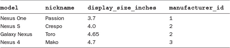
Now, each device has a manufacturer_id that references a row in the manufacturer table.
Now that the two tables are defined and populated, a JOIN between them can be performed in a SELECT statement. Listing 2.20 shows a SELECT statement that combines all the data from the two tables.
Listing 2.20 Joining the Tables with JOIN
SELECT model, nickname, display_size_inches, short_name, long_name
FROM device
JOIN manufacturer
ON (device.manufacturer_id = manufacturer.id);
The SELECT statement in Listing 2.20 returns the rows from both the device and manufacturer tables in the projection. The FROM clause in the SELECT statement is where the JOIN operation happens.
The following code fragment indicates that the device and manufacturer tables should be joined where the manufacturer_id from the device table matches the value of the id column from the manufacturer table:
FROM device JOIN manufacturer ON (device.manufacturer_id = manufacturer.id)
The outcome of the SELECT statement in Listing 2.20 is a single result that combines the data from two different tables as if they were a single table.
Summary
SQL contains different types of statements to perform operations on a database. Data Definition Language (DDL) includes the SQL commands and statements needed to define a schema for a database using various database objects such as tables, views, triggers, and indexes. The operations included in DDL are CREATE, ALTER, and DROP.
Data Manipulation Language (DML) contains SQL language features needed to work with the data in tables. These include the INSERT, UPDATE, and DELETE statements.
Once a database has been defined and populated with data, the SELECT statement can be used to query the database. A query defines which table columns should be returned as the result along with which rows from the database should be selected for inclusion in the result set.
Chapter 3, “An Introduction to SQLite,” goes into more details about SQLite, which is the SQL database implementation included in Android.