© Ramcharan Kakarla, Sundar Krishnan and Sridhar Alla 2021
R. Kakarla et al.Applied Data Science Using PySparkhttps://doi.org/10.1007/978-1-4842-6500-0_8

8. Machine Learning Flow and Automated Pipelines

Ramcharan Kakarla1  , Sundar Krishnan1 and Sridhar Alla2
(1)
Philadelphia, PA, USA
(2)
New Jersey, NJ, USA
 

Putting a model into production is one of the most challenging tasks in the data science world. It is one of those last-mile problems that persists in many organizations. Although there are many tools for managing workflows, as the organization matures its needs change, and managing existing models can become a herculean task. When we take a step back and analyze why it is so challenging, we can see that it is because of the structure that exists in most organizations. There is an engineering team that maintains the production platform. There is a gap between the data science toolset and the production platforms. Some of the data science work can be developed in Jupyter Notebook, with little consideration given to the cloud environment. Some of the data flows are created locally with limited scaling. Such applications tend to falter with large amounts of data. Best practices that exist in the software development cycle don’t stick well with the machine learning lifecycle because of the variety of tasks involved. The standard is mainly defined by the data science team in the organization. Also, rapid developments in the field are leaving vacuums with respect to the management and deployment of models.

The goal of this chapter is to explore the tools available for managing and deploying data science pipelines. We will walk you through some of the tools available in the industry and demonstrate with an example how to construct an automated pipeline. We will use all the concepts that we have learned so far to construct these pipelines. By the end of this chapter, you will have learned how to build the machine learning blocks and automate them in coherence with custom data preprocessing.

We will cover the following topics in this chapter:
  • MLflow. We will introduce MLflow as well as its components and advantages, followed by a demonstration. In the first half, our focus will be on the installation and introduction of concepts. In the second half, we will focus on implementing a model in MLflow.

  • Automated machine learning pipelines. We will introduce the concept of designing and implementing automated ML frameworks in PySpark. The first half of the section is heavily focused on implementation, and the second half focuses on the outputs generated from the pipeline.

MLflow

With the knowledge obtained from previous chapters, we know how to build individual supervised and unsupervised models. Often times we would try multiple iterations before picking the best model. How do we keep track of all the experiments and the hyperparameters we used? How can we reproduce a particular result after multiple experiments? How do we move a model into production when there are multiple deployment tools and environments? Is there a way to better manage the machine learning workflow and share work with the wider community? These are some of the questions that you will have after you are comfortable building models in PySpark. Databricks has built a tool named MLflow that can gracefully handle some of the preceding questions while managing the machine learning workflow. MLflow is designed to be open interface and open source. People often tend to go back and forth between experimentation and adding new features to the model. MLflow handles such experimentation with ease. It is built around REST APIs that can be consumed easily by multiple tools. This framework also makes it easy to add existing machine learning blocks of code. Its open source nature makes it makes it easy to share the workflows and models across different teams. In short, MLflow offers a framework to manage the machine learning lifecycle, including experimentation, reproducibility, deployment, and central model registry.

MLflow components are shown in Figure 8-1 and described in the following list.
../images/500182_1_En_8_Chapter/500182_1_En_8_Fig1_HTML.png
Figure 8-1

MLflow components

  • Tracking: Aids in recording, logging code, configurations, data, and results. It also gives a mechanism to query experiments.

  • Projects: This component of MLflow helps in bundling the machine learning code in a format for easy replication on multiple platforms.

  • Models: This assists in deploying machine learning code in diverse environments.

  • Model Registry: This component acts like a repository in which to store, manage, and search models.

This framework opens the tunnel for data engineers and data scientists to collaborate and efficiently build data pipelines. It also provides the ability to consume and write data from and to many different systems. It opens up a common framework for working with both structured and unstructured data in data lakes as well as on batch streaming platforms.

This may look abstract for first-time users. We will walk you through an example of how these components can be useful and implemented. For this purpose of illustration, let us take the same bank dataset we used in Chapter 6.

MLflow Code Setup and Installation

In this section, we will walk through the code changes necessary to support MLflow, along with its installation. We will be using a PySpark Docker version for all demonstrations. There are two main steps to get MLflow up and running, as follows:
  • Code/script changes

  • Docker side changes and MLflow server installation

Code changes are minimal. We have to add a few MLflow functions to existing machine learning code to accommodate MLflow.

Regular code works well for building a simple random forest model, but what if I want to know the Receiver Operating Characteristic (ROC)/other metrics (accuracy, misclassification, etc) by changing the input variables or any hyperparameter settings? Well, if it’s a single change we can record each run in Excel, but this is not an efficient way of tracking our experiments. As data science professionals, we run hundreds of experiments, especially in the model fine-tuning phase. Is there a better way of capturing and annotating these results and logs? Yes, we can do it via the MLflow tracking feature. Now, let’s rewrite a simple random forest model code, adding MLflow components. Changes in the code are highlighted in bold.

Note

We will save the following code as .py and run via Docker after installing MLflow.

# Import libraries
import pyspark
from pyspark.sql import SparkSession
import mlflow
import mlflow.spark
import sys
import time
from pyspark.ml.classification import RandomForestClassifier
from pyspark.ml.evaluation import BinaryClassificationEvaluator
Observe we have imported the libraries related to MLflow that allow the user to use PySpark. Note MLflow supports a variety of languages and packages, including Spark and Python, with extended support for packages like scikitlearn and tensorflow.
spark = SparkSession.builder.appName("mlflow_example").getOrCreate()
filename = "/home/jovyan/work/bank-full.csv"
target_variable_name = "y"
from pyspark.sql import functions as F
df = spark.read.csv(filename, header=True, inferSchema=True, sep=';')
df = df.withColumn('label', F.when(F.col("y") == 'yes', 1).otherwise(0))
df = df.drop('y')
train, test = df.randomSplit([0.7, 0.3], seed=12345)
for k, v in df.dtypes:
    if v not in ['string']:
        print(k)
df = df.select(['age', 'balance', 'day', 'duration', 'campaign', 'pdays', 'previous', 'label'])
from pyspark.ml.feature import VectorAssembler
from pyspark.ml import Pipeline
def assemble_vectors(df, features_list, target_variable_name):
    stages = []
    #assemble vectors
    assembler = VectorAssembler(inputCols=features_list, outputCol="features")
    stages = [assembler]
    #select all the columns + target + newly created 'features' column
    selectedCols = [target_variable_name, 'features']
    #use pipeline to process sequentially
    pipeline = Pipeline(stages=stages)
    #assembler model
    assembleModel = pipeline.fit(df)
    #apply assembler model on data
    df = assembleModel.transform(df).select(selectedCols)
    return df
#exclude target variable and select all other feature vectors
features_list = df.columns
#features_list = char_vars #this option is used only for ChiSqselector
features_list.remove('label')
# apply the function on our DataFrame
assembled_train_df = assemble_vectors(train, features_list, 'label')
assembled_test_df = assemble_vectors(test, features_list, 'label')
print(sys.argv[1])
print(sys.argv[2])
These are the system arguments we intend to change in each experiment. We will pass this as system arguments when we execute this script. Here we used maxBins and maxDepth. You are free to include any other variable changes you want to log across the script.
from pyspark.ml.classification import RandomForestClassifier
from pyspark.ml.evaluation import BinaryClassificationEvaluator
maxBinsVal = float(sys.argv[1]) if len(sys.argv) > 3 else 20
maxDepthVal = float(sys.argv[2]) if len(sys.argv) > 3 else 3
In the following step, we are initializing the machine learning code part with MLflow since our tracking variables of interest are within this scope. You can modify the scope as intended depending upon the use case.
with mlflow.start_run():
    stages_tree=[]
    classifier = RandomForestClassifier(labelCol = 'label',featuresCol = 'features',maxBins=maxBinsVal, maxDepth=maxDepthVal)
    stages_tree += [classifier]
    pipeline_tree=Pipeline(stages=stages_tree)
    print('Running RFModel')
    RFmodel = pipeline_tree.fit(assembled_train_df)
    print('Completed training RFModel')
    predictions = RFmodel.transform(assembled_test_df)
    evaluator = BinaryClassificationEvaluator()
    print("Test Area Under ROC: " + str(evaluator.evaluate(predictions, {evaluator.metricName: "areaUnderROC"})))
    mlflow.log_param("maxBins", maxBinsVal)
    mlflow.log_param("maxDepth", maxDepthVal)
    mlflow.log_metric("ROC", evaluator.evaluate(predictions, {evaluator.metricName: "areaUnderROC"}))
    mlflow.spark.log_model(RFmodel,"spark-model")

In the preceding snippet of code, we added log_param and log_metric to capture the pieces of information we want to keep tabs on. Also note we are logging the model using the mlflow.spark.log_model function , which helps in saving the model on the MLflow backend. This is an optional statement, but it is handy if you want to register the model from MLflow. With minimal changes in code, we are able to accommodate an existing model with MLflow components. Why is it so important? Tracking the change in parameters and metrics can become challenging with hundreds of experiments staged over multiple days. We will need to save the preceding code as a Python file. We will be using a Spark submit to execute this PySpark code. In this illustration, we saved it as Chapter9_mlflow_example.py.

Moving on to part two of MLflow setup, it is time to initiate the Docker container using the following command. Recall this is the same PySpark Docker image we demonstrated in Chapter 1. We also have to save the preceding Python file in the same local path that we are mapping to the Docker container. The following Docker initiation code and its local mapping works for Mac; for Windows, please change your path appropriately.
docker run -it -p 5000:5000 -v /Users/ramcharankakarla/demo_data/:/home/jovyan/work/ jupyter/pyspark-notebook:latest bash
Note

MLflow by default uses port 5000.

As we enter into Docker, we like to change the path to work (cd /home/jovyan/work/) since all our local information, including the Python file Chapter9_mlflow_example.py, is mapped there. The following two commands help you to change directory and see the contents available on the work directory in Docker.
cd work
ls
Make sure you see the Python file in this path. Often times the Docker image may not contain the MLflow. It is a good practice to verify if the MLflow package is available in the image by using pip freeze|grep mlflow. If MLflow is not available, add the package using the following command:
pip install mlflow
The next step is to initialize the MLflow server. This server is the backend to the user interface and captures all the information pertaining to the experiments. It can be initiated using the following command. Note that we are running this command in the background.
mlflow server --backend-store-uri sqlite:///mlflow.db --default-artifact-root /home/jovyan/work --host 0.0.0.0 --port 5000 &
Note the parameters here contain backend-store-uri and default-artifact-root. Backend-store-uri is mandatory if we want to register or log any models. We used a default sqlite MLflow data base (db) here for demonstration. This can be any other backend store, including file-based and database-backend stores. This powers the querying capability of MLflow. Artifact root is the location of the artifact store and is suitable for large data. This is where all the artifacts pertaining to the experiments reside. By default the location of --default-artifact-root is set to ./mlruns. You can override this setting by giving an appropriate location. Different artifact stores are supported by MLflow including, the following:
  • HDFS

  • NFS

  • FTP server

  • SFTP server

  • Google Cloud storage (GCS)

  • Azure Blob storage

  • Amazon S3

It is important to specify the artifact URI when creating an experiment, or else the client and server will refer to different physical locations; i.e., the same path on different disk locations (Table 8-1).
Table 8-1

Storage Types

Storage Type

URI Format

FTP

ftp://user:pass@host/path/to/directory

SFTP

sftp://user@host/path/to/directory

NFS

/mnt/nfs

HDFS

hdfs://<host>:<port>/<path>

Azure

wasbs://<container>@<storage-account>.blob.core.windows.net/<path>

Amazon S3

s3://<bucket>/<path>

There are additional settings needing to be authenticated for a few storage types. For S3, credentials can be obtained from environment variables AWS_ACCESS_KEY_ID and AWS_SECRET_ACCESS_KEY or from the IAM profile.

MLflow User Interface Demonstration

In this section, we will walk through the MLflow user interface with an example we discussed in the previous section. The following are running the script we saved earlier with three different settings:
MLFLOW_TRACKING_URI="http://0.0.0.0:5000" spark-submit --master local[*] /home/jovyan/work/Chapter9_mlflow_example.py 16 3  --spark_autolog True
MLFLOW_TRACKING_URI="http://0.0.0.0:5000" spark-submit --master local[*] /home/jovyan/work/Chapter9_mlflow_example.py 16 5  --spark_autolog True
MLFLOW_TRACKING_URI="http://0.0.0.0:5000" spark-submit --master local[*] /home/jovyan/work/Chapter9_mlflow_example.py 32 5  --spark_autolog True
Once we finish running the preceding three commands, we can proceed with initiating the MLflow user interface. On any web browser, navigate to http://0.0.0.0:5000. You will see the MLflow user interface shown in Figure 8-2.
../images/500182_1_En_8_Chapter/500182_1_En_8_Fig2_HTML.jpg
Figure 8-2

MLflow UI

As you can see, the user interface has all the information formatted into experiments and models. We can make any annotations or notes using the notes options pertaining to each of the runs within each experiment. This framework gives us the ability to manage and run multiple experiments with multiple runs. We also have an option to filter the runs based on parameter settings. This is extremely useful in a machine learning lifecycle because, unlike the software development lifecycle, we tend to iterate between old and newer versions based on the stability and accuracy of the models.

There is also detailed row-level information on each run. We can drill down and compare this information across many experiments. For our illustration, we have only used a single metric, but in a real-world scenario, we may also want to capture accuracy, misclassification, lift, and KS statistics for each run. We could then compare and sort each iteration based on a metric that is acceptable based on business need.

When we select a couple of iterations from the prior executions, observe the Compare button is active; it is greyed out in Figure 8-2. When we click on Compare it will compare these two iterations and also give prepared graphs on how metrics are varying across different runs (Figure 8-3). In the preceding code we have explicitly set the log metrics. From version 3 of Spark there is an option for automatic logging.
../images/500182_1_En_8_Chapter/500182_1_En_8_Fig3_HTML.jpg
Figure 8-3

MLflow UI comparison of runs

Observe the window in Figure 8-4; MLflow autogenerates the runids. We can compare multiple runs in an experiment using this feature. When we have enough data points, we can visually pick the model runs that are giving the best performance. We can also observe how the model performance can vary by changing the parameters.
../images/500182_1_En_8_Chapter/500182_1_En_8_Fig4_HTML.jpg
Figure 8-4

MLflow UI comparison window

If we go back to the homepage in the MLflow UI and click on any run, it will give us more information about the model run, as shown in Figure 8-5. This Run window also gives us the handy feature of registering the model. Registering a model will make it available for scoring. There are multiple other features that will open up upon registering the model.
../images/500182_1_En_8_Chapter/500182_1_En_8_Fig5_HTML.jpg
Figure 8-5

MLflow UI Run window

Clicking the spark-model file in the Artifacts section will open up the next window. This will contain all the metadata information of the model required for running it, as shown in Figure 8-6.
../images/500182_1_En_8_Chapter/500182_1_En_8_Fig6_HTML.jpg
Figure 8-6

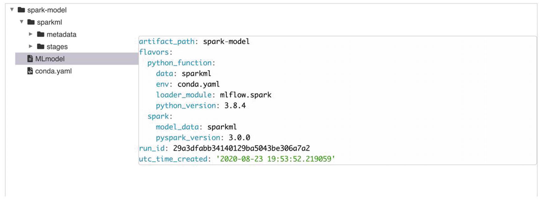
MLflow UI model information

If you click the root folder it will give an option to register the model in the metadata, as shown in Figure 8-7.
../images/500182_1_En_8_Chapter/500182_1_En_8_Fig7_HTML.jpg
Figure 8-7

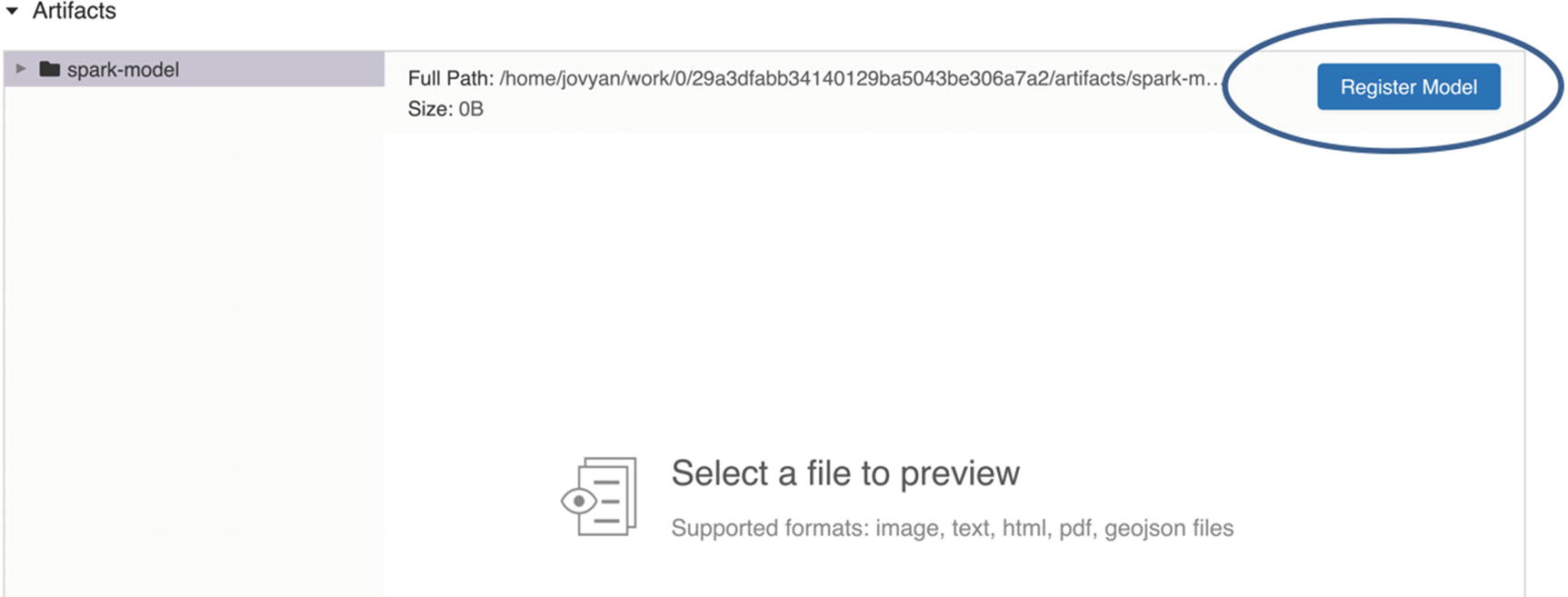
MLflow UI model registration

Adding the model as shown in Figure 8-8 pushes the model into the Models tab. You can verify this by navigating to the Models tab at the top (Figure 8-9).
../images/500182_1_En_8_Chapter/500182_1_En_8_Fig8_HTML.jpg
Figure 8-8

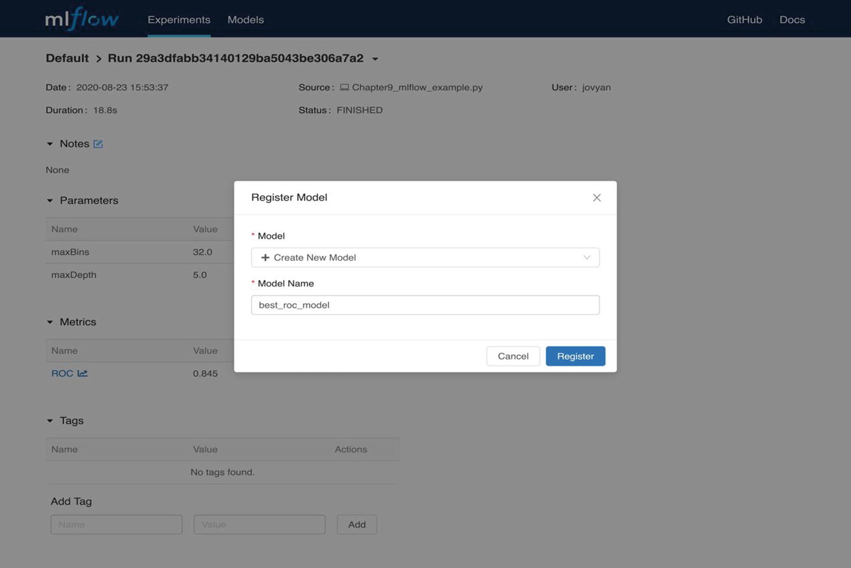
MLflow UI Registration window

../images/500182_1_En_8_Chapter/500182_1_En_8_Fig9_HTML.jpg
Figure 8-9

MLflow Models tab

On clicking the model name, you will navigate to a new window with detailed model information. The new window will also give options to push the model into three different environments, as shown in Figure 8-10.
  • Staging

  • Production

  • Archived

../images/500182_1_En_8_Chapter/500182_1_En_8_Fig10_HTML.jpg
Figure 8-10

MLflow model environments

This helps in effectively managing the model lifecycle by moving models to different environments as we transition from model development to the end of the model lifecycle.

Well, all this is great, but how can we score new data from these pipelines? When we click on either the run or the model information, we get the full path of the model metadata information, represented in Figure 8-7. We can use this metadata to score any new data. There are multiple ways this can be achieved. Let us write a simple code to prepare data for scoring, and we will use the best_roc_model shown in Figure 8-10. We will save the following code as a Python file and run it via spark-submit in Docker.
#Importing necessary libraries
import mlflow
import mlflow.spark
import sys
from pyspark.sql import SparkSession
spark = SparkSession.builder.appName("mlflow_predict").getOrCreate()
filename = "/home/jovyan/work/bank-full.csv"
target_variable_name = "y"
from pyspark.sql import functions as F
df = spark.read.csv(filename, header=True, inferSchema=True, sep=';')
df = df.withColumn('label', F.when(F.col("y") == 'yes', 1).otherwise(0))
df = df.drop('y')
train, test = df.randomSplit([0.7, 0.3], seed=12345)
for k, v in df.dtypes:
    if v not in ['string']:
        print(k)
df = df.select(['age', 'balance', 'day', 'duration', 'campaign', 'pdays', 'previous', 'label'])
from pyspark.ml.feature import VectorAssembler
from pyspark.ml import Pipeline
# assemble individual columns to one column - 'features'
def assemble_vectors(df, features_list, target_variable_name):
    stages = []
    #assemble vectors
    assembler = VectorAssembler(inputCols=features_list, outputCol="features")
    stages = [assembler]
    #select all the columns + target + newly created 'features' column
    selectedCols = [target_variable_name, 'features']
    #use pipeline to process sequentially
    pipeline = Pipeline(stages=stages)
    #assembler model
    assembleModel = pipeline.fit(df)
    #apply assembler model on data
    df = assembleModel.transform(df).select(selectedCols)
    return df
#exclude target variable and select all other feature vectors
features_list = df.columns
#features_list = char_vars #this option is used only for ChiSqselector
features_list.remove('label')
# apply the function on our dataframe
assembled_test_df = assemble_vectors(test, features_list, 'label')
print(sys.argv[1])
# model information from argument
model_uri=sys.argv[1]
print("model_uri:", model_uri)
model = mlflow.spark.load_model(model_uri)
print("model.type:", type(model))
predictions = model.transform(assembled_test_df)
print("predictions.type:", type(predictions))
predictions.printSchema()
df = predictions.select('rawPrediction','probability', 'label', 'features')
df.show(5, False)
This code is a simple pipeline. We also have the flexibility of wrapping the scoring function as a simple udf as well. After saving the code, we need to run the following command in Docker for results:
spark-submit --master local[*] Chapter9_predict_spark.py /home/jovyan/work/0/29a3dfabb34140129ba5043be306a7a2/artifacts/spark-model
This will give us the output shown in Figure 8-11.
../images/500182_1_En_8_Chapter/500182_1_En_8_Fig11_HTML.jpg
Figure 8-11

MLflow model scoring output

All the preceding content and codes are specified in Spark. There are multiple other flavors that MLflow supports. We can serialize the preceding pipeline in the mleap flavor, which is a project to host Spark pipelines without a Spark context for smaller datasets where we don’t need any distributed computing. MLflow also has the capability to publish the code to GitHub in the MLflow project format, making it easy for anyone to run the code.

Automated Machine Learning Pipelines

The machine learning lifecycle is an iterative process. We often tend to go back and forth tuning parameters, inputs and data pipelines. This can quickly get cumbersome with the number of data management pipelines. Creating automated pipelines can save a significant amount of time. From all the earlier chapters we have learned data manipulations, algorithms, and modeling techniques. Now, let us put them all together to create an automated PySpark flow that can generate baseline models for quick experimentation.

For this experiment, we will use a churn dataset from Kaggle (https://www.kaggle.com/shrutimechlearn/churn-modelling#Churn_Modelling.csv). This banking dataset contains data about attributes of customers and who has churned. Our objective is to identify customers who will churn based on given attributes. Table 8-2 lists the attributes.
Table 8-2

Metadata

Column

Description

RowNumber

Identifier

CustomerId

Unique ID for customer

Surname

Customer's last name

Credit score

Credit score of the customer

Geography

The country to which the customer belongs

Gender

Male or female

Age

Age of customer

Tenure

Number of years for which the customer has been with the bank

Balance

Bank balance of the customer

NumOfProducts

Number of bank products the customer is utilizing

HasCrCard

Binary flag for whether the customer holds a credit card with the bank or not

IsActiveMember

Binary flag for whether the customer is an active member with the bank or not

EstimatedSalary

Estimated salary of the customer in dollars

Exited

Binary flag: 1 if the customer closed account with bank and 0 if the customer is retained

Pipeline Requirements and Framework

When designing any pipeline, it is imperative to define what outputs and requirements we expect. First, let us define the outputs that we think are necessary. Since we are tackling a binary target, it would be nice to have the following outputs:
  • KS: Kolmogorov-Smirnov test is a measure of separation between goods and the bads. Higher is better..

  • ROC: (ROC) Curve is a way to compare diagnostic tests. It is a plot of the true positive rate against the false positive rate. Higher is better.

  • Accuracy: (true positives+true negatives)/ (true positives+true negatives+false positives+false negatives). Higher is better.

Now, let’s list the requirements for an automated model building tool.
  • Module should be able to handle the missing values and categorical values by itself.

  • We also prefer the module to take care of variable selection.

  • We also want this module to test out multiple algorithms before selecting the final variables.

  • Let the module compare different algorithms based on preferred metric and select the champion and challenger models for us.

  • It would be handy if it could remove certain variables by prefix or suffix or by variable names. This can power multiple iterations and tweak input variables.

  • Module should be able to collect and store all the output metrics and collate them to generate documents for later reference.

  • Finally , it would be nice if the module could save the model objects and autogenerate the scoring codes so we can just deploy the selected model.

How are we writing these requirements? Remember we discussed the CRISP–DM framework in Chapter 3 (Figure 8-12)? We are making use of this framework here as our architecture blueprint.
../images/500182_1_En_8_Chapter/500182_1_En_8_Fig12_HTML.png
Figure 8-12

CRISP–DM

Now, these are a lot of requirements and can quickly become overwhelming if not handled properly. We defined the outputs and requirements, but what will be our expected inputs? Probably a dataset either from a datastore or a flatfile. With this specified information, we can start building the pipelines step-by-step by breaking the code into logical steps. This will be a code-intensive chapter, and you will be able to use this module and create your own baseline automated models. We will break tasks into subtasks in each of the logical steps. These can be broadly divided into the following:
  • Data manipulations

  • Feature selection

  • Model building

  • Metrics calculation

  • Validation and plot generation

  • Model selection

  • Score code creation

  • Collating results

  • Framework to handle all the preceding steps

Data Manipulations

In this section, we will define some commonly used functions for handling the data, such as the following:
  • Missing value percentage calculations

  • Metadata categorization of input data

  • Handling categorical data using label encoders

  • Imputing missing values

  • Renaming categorical columns

  • Combining features and labels

  • Data splitting to training, testing, and validation

  • Assembling vectors

  • Scaling input variables

from pyspark.ml.feature import StringIndexer
from pyspark.ml import Pipeline
from pyspark.sql import *
from pyspark.sql.types import *
from pyspark.sql import functions as F
from pyspark.ml.feature import IndexToString
from pyspark.sql.functions import col
from pyspark.ml.feature import StandardScaler
from pyspark.ml.feature import VectorAssembler
#    1. Missing value calculation
def missing_value_calculation(X, miss_per=0.75):
    missing = X.select([F.count(F.when(F.isnan(c) | F.col(c).isNull(), c)).alias(c) for c in X.columns])
    missing_len = X.count()
    final_missing = missing.toPandas().transpose()
    final_missing.reset_index(inplace=True)
    final_missing.rename(columns={0:'missing_count'},inplace=True)
    final_missing['missing_percentage'] = final_missing['missing_count']/missing_len
    vars_selected = final_missing['index'][final_missing['missing_percentage'] <= miss_per]
    return vars_selected
#    2. Metadata categorization
def identify_variable_type(X):
    l = X.dtypes
    char_vars = []
    num_vars = []
    for i in l:
        if i[1] in ('string'):
            char_vars.append(i[0])
        else:
            num_vars.append(i[0])
    return char_vars, num_vars
#    3. Categorical to Numerical using label encoders
def categorical_to_index(X, char_vars):
    chars = X.select(char_vars)
    indexers = [StringIndexer(inputCol=column, outputCol=column+"_index",handleInvalid="keep") for column in chars.columns]
    pipeline = Pipeline(stages=indexers)
    char_labels = pipeline.fit(chars)
    X = char_labels.transform(X)
    return X, char_labels
#    4. Impute Numerical columns with a specific value . The default is set to 0.
def numerical_imputation(X,num_vars, impute_with=0):
    X = X.fillna(impute_with,subset=num_vars)
    return X
#    5. Rename categorical columns
def rename_columns(X, char_vars):
    mapping = dict(zip([i+ '_index' for i in char_vars], char_vars))
    X = X.select([col(c).alias(mapping.get(c, c)) for c in X.columns])
    return X
#    6. Combining features and labels
def join_features_and_target(X, Y):
    X = X.withColumn('id', F.monotonically_increasing_id())
    Y = Y.withColumn('id', F.monotonically_increasing_id())
    joinedDF = X.join(Y,'id','inner')
    joinedDF = joinedDF.drop('id')
    return joinedDF
#    7. Data splitting to training, testing, and validation
def train_valid_test_split(df, train_size=0.4, valid_size=0.3,seed=12345):
    train, valid, test = df.randomSplit([train_size, valid_size,1-train_size-valid_size], seed=12345)
    return train,valid,test
#    8. Assembling vectors
def assembled_vectors(train,list_of_features_to_scale,target_column_name):
    stages = []
    assembler = VectorAssembler(inputCols=list_of_features_to_scale, outputCol="features")
    stages=[assembler]
    selectedCols = [target_column_name,'features'] + list_of_features_to_scale
    pipeline = Pipeline(stages=stages)
    assembleModel = pipeline.fit(train)
    train = assembleModel.transform(train).select(selectedCols)
    return train
#    9. Scaling input variables
def scaled_dataframes(train,valid,test,list_of_features_to_scale,target_column_name):
    stages = []
    assembler = VectorAssembler(inputCols=list_of_features_to_scale, outputCol="assembled_features")
    scaler = StandardScaler(inputCol=assembler.getOutputCol(), outputCol="features")
    stages=[assembler,scaler]
    selectedCols = [target_column_name,'features'] + list_of_features_to_scale
    pipeline = Pipeline(stages=stages)
    pipelineModel = pipeline.fit(train)
    train = pipelineModel.transform(train).select(selectedCols)
    valid = pipelineModel.transform(valid).select(selectedCols)
    test = pipelineModel.transform(test).select(selectedCols)
    return train, valid, test, pipelineModel

Feature Selection

This module shortlists the variables and selects the top variables that are the most predictive features. It uses random forests to identify the top variables.
import pandas as pd
import matplotlib
matplotlib.use('Agg')
import matplotlib.pyplot as plt
# The module below is used to draw the feature importance plot
def draw_feature_importance(user_id, mdl_ltrl, importance_df):
    importance_df = importance_df.sort_values('Importance_Score')
    plt.figure(figsize=(15,15))
    plt.title('Feature Importances')
    plt.barh(range(len(importance_df['Importance_Score'])), importance_df['Importance_Score'], align="center")
    plt.yticks(range(len(importance_df['Importance_Score'])), importance_df['name'])
    plt.ylabel('Variable Importance')
    plt.savefig('/home/' + user_id + '/' + 'mla_' + mdl_ltrl + '/' + 'Features selected for modeling.png', bbox_inches="tight")
    plt.close()
    return None
# The module below is used to save the feature importance as an Excel file
def save_feature_importance(user_id, mdl_ltrl, importance_df):
    importance_df.drop('idx',axis=1,inplace=True)
    importance_df = importance_df[0:30]
    importance_df.to_excel('/home/' + user_id + '/' + 'mla_' + mdl_ltrl + '/' + 'feature_importance.xlsx')
    draw_feature_importance(user_id, mdl_ltrl, importance_df)
    return None
# The following module is used to calculate the feature importance for each variable based on the Random Forest output. The feature importance is used to reduce the final variable list to 30.
def ExtractFeatureImp(featureImp, dataset, featuresCol):
    """
    Takes in a feature importance from a random forest / GBT model and maps it to the column names
    Output as a pandas DataFrame for easy reading
    rf = RandomForestClassifier(featuresCol="features")
    mod = rf.fit(train)
    ExtractFeatureImp(mod.featureImportances, train, "features")
    """
    list_extract = []
    for i in dataset.schema[featuresCol].metadata["ml_attr"]["attrs"]:
        list_extract = list_extract + dataset.schema[featuresCol].metadata["ml_attr"]["attrs"][i]
    varlist = pd.DataFrame(list_extract)
    varlist['Importance_Score'] = varlist['idx'].apply(lambda x: featureImp[x])
    return(varlist.sort_values('Importance_Score', ascending = False))

Model Building

In this module, we define multiple algorithm functions that support binary targets, including logistic regression, random forests, gradient boosting, and neural nets.
from pyspark.ml.classification import LogisticRegression
from pyspark.ml.classification import LogisticRegressionModel
# from sklearn.externals import joblib
import joblib
def logistic_model(train, x, y):
    lr = LogisticRegression(featuresCol = x, labelCol = y, maxIter = 10)
    lrModel = lr.fit(train)
    return lrModel
from pyspark.ml.classification import RandomForestClassifier
from pyspark.ml.classification import RandomForestClassificationModel
def randomForest_model(train, x, y):
    rf = RandomForestClassifier(featuresCol = x, labelCol = y, numTrees=10)
    rfModel = rf.fit(train)
    return rfModel
from pyspark.ml.classification import GBTClassifier
from pyspark.ml.classification import GBTClassificationModel
def gradientBoosting_model(train, x, y):
    gb = GBTClassifier(featuresCol = x, labelCol = y, maxIter=10)
    gbModel = gb.fit(train)
    return gbModel
from pyspark.ml.classification import DecisionTreeClassifier
from pyspark.ml.classification import DecisionTreeClassificationModel
def decisionTree_model(train, x, y):
    dt = DecisionTreeClassifier(featuresCol = x, labelCol = y, maxDepth=5)
    dtModel = dt.fit(train)
    return dtModel
from pyspark.ml.classification import MultilayerPerceptronClassifier
from pyspark.ml.classification import MultilayerPerceptronClassificationModel
def neuralNetwork_model(train, x, y, feature_count):
    layers = [feature_count, feature_count*3, feature_count*2, 2]
    mlp = MultilayerPerceptronClassifier(featuresCol = x, labelCol = y, maxIter=100, layers=layers, blockSize=512,seed=12345)
    mlpModel = mlp.fit(train)
    return mlpModel

Metrics Calculation

The following module calculates the model metrics including KS, ROC, and accuracy.
from pyspark.sql.types import DoubleType
from pyspark.sql import *
from pyspark.sql.functions import desc
from pyspark.sql.functions import udf
from pyspark.sql import functions as F
import sys
import time
# import __builtin__ as builtin
import builtins
from pyspark.ml.evaluation import BinaryClassificationEvaluator
from pyspark.ml.feature import QuantileDiscretizer
import numpy
import numpy as np
from pyspark import SparkContext,HiveContext,Row,SparkConf
spark = SparkSession.builder.appName("MLA_metrics_calculator").enableHiveSupport().getOrCreate()
spark.sparkContext.setLogLevel('ERROR')
sc = spark.sparkContext
def highlight_max(data, color="yellow"):
    '''
    highlight the maximum in a Series or DataFrame
    '''
    attr = 'background-color: {}'.format(color)
    if data.ndim == 1:  # Series from .apply(axis=0) or axis=1
        is_max = data == data.max()
        return [attr if v else '' for v in is_max]
    else:  # from .apply(axis=None)
        is_max = data == data.max().max()
        return pd.DataFrame(np.where(is_max, attr, ''),index=data.index, columns=data.columns)
def calculate_metrics(predictions,y,data_type):
    start_time4 = time.time()
    # Calculate ROC
    evaluator = BinaryClassificationEvaluator(labelCol=y,rawPredictionCol='probability')
    auroc = evaluator.evaluate(predictions,{evaluator.metricName: "areaUnderROC"})
    print('AUC calculated',auroc)
    selectedCols = predictions.select(F.col("probability"), F.col('prediction'), F.col(y)).rdd.map(lambda row: (float(row['probability'][1]), float(row['prediction']), float(row[y]))).collect()
    y_score, y_pred, y_true = zip(*selectedCols)
    # Calculate Accuracy
    accuracydf=predictions.withColumn('acc',F.when(predictions.prediction==predictions[y],1).otherwise(0))
    accuracydf.createOrReplaceTempView("accuracyTable")
    RFaccuracy=spark.sql("select sum(acc)/count(1) as accuracy from accuracyTable").collect()[0][0]
    print('Accuracy calculated',RFaccuracy)
#     # Build KS Table
    split1_udf = udf(lambda value: value[1].item(), DoubleType())
    if data_type in ['train','valid','test','oot1','oot2']:
        decileDF = predictions.select(y, split1_udf('probability').alias('probability'))
    else:
        decileDF = predictions.select(y, 'probability')
    decileDF=decileDF.withColumn('non_target',1-decileDF[y])
    window = Window.orderBy(desc("probability"))
    decileDF = decileDF.withColumn("rownum", F.row_number().over(window))
    decileDF.cache()
    decileDF=decileDF.withColumn("rownum",decileDF["rownum"].cast("double"))
    window2 = Window.orderBy("rownum")
    RFbucketedData=decileDF.withColumn("deciles", F.ntile(10).over(window2))
    RFbucketedData = RFbucketedData.withColumn('deciles',RFbucketedData['deciles'].cast("int"))
    RFbucketedData.cache()
    #a = RFbucketedData.count()
    #print(RFbucketedData.show())
    ## to pandas from here
    print('KS calculation starting')
    target_cnt=RFbucketedData.groupBy('deciles').agg(F.sum(y).alias('target')).toPandas()
    non_target_cnt=RFbucketedData.groupBy('deciles').agg(F.sum("non_target").alias('non_target')).toPandas()
    overall_cnt=RFbucketedData.groupBy('deciles').count().alias('Total').toPandas()
    overall_cnt = overall_cnt.merge(target_cnt,on='deciles',how='inner').merge(non_target_cnt,on='deciles',how='inner')
    overall_cnt=overall_cnt.sort_values(by='deciles',ascending=True)
    overall_cnt['Pct_target']=(overall_cnt['target']/overall_cnt['count'])*100
    overall_cnt['cum_target'] = overall_cnt.target.cumsum()
    overall_cnt['cum_non_target'] = overall_cnt.non_target.cumsum()
    overall_cnt['%Dist_Target'] = (overall_cnt['cum_target'] / overall_cnt.target.sum())*100
    overall_cnt['%Dist_non_Target'] = (overall_cnt['cum_non_target'] / overall_cnt.non_target.sum())*100
    overall_cnt['spread'] = builtins.abs(overall_cnt['%Dist_Target']-overall_cnt['%Dist_non_Target'])
    decile_table=overall_cnt.round(2)
    print("KS_Value =", builtins.round(overall_cnt.spread.max(),2))
    decileDF.unpersist()
    RFbucketedData.unpersist()
    print("Metrics calculation process Completed in : "+ " %s seconds" % (time.time() - start_time4))
    return auroc,RFaccuracy,builtins.round(overall_cnt.spread.max(),2), y_score, y_pred, y_true, overall_cnt

Validation and Plot Generation

This module generates the various plots, including ROC, confusion matrix, and KS. Model validation is also done as part of this module.
import matplotlib
matplotlib.use('Agg')
import matplotlib.pyplot as plt
from sklearn import metrics
import glob
import os
import pandas as pd
import seaborn as sns
from pandas import ExcelWriter
from metrics_calculator import *
# Generate ROC chart
def draw_roc_plot(user_id, mdl_ltrl, y_score, y_true, model_type, data_type):
    fpr, tpr, thresholds = metrics.roc_curve(y_true, y_score, pos_label = 1)
    roc_auc = metrics.auc(fpr,tpr)
    plt.title(str(model_type) + ' Model - ROC for ' + str(data_type) + ' data' )
    plt.plot([0, 1], [0, 1], 'r--')
    plt.plot(fpr, tpr, label = 'AUC = %0.2f' % roc_auc)
    plt.xlabel('False Positive Rate (1 - Specificity)')
    plt.ylabel('True Positive Rate (Sensitivity)')
    plt.legend(loc = 'lower right')
    print('/home/' + user_id + '/' + 'mla_' + mdl_ltrl + '/' + str(model_type) + '/' + str(model_type) + ' Model - ROC for ' + str(data_type) + ' data.png')
    plt.savefig('/home/' + user_id + '/' + 'mla_' + mdl_ltrl + '/' + str(model_type) + '/' + str(model_type) + ' Model - ROC for ' + str(data_type) + ' data.png', bbox_inches="tight")
    plt.close()
# Generate KS chart
def draw_ks_plot(user_id, mdl_ltrl, model_type):
    writer = ExcelWriter('/home/' + user_id + '/' + 'mla_' + mdl_ltrl + '/' + str(model_type) + '/KS_Charts.xlsx')
    for filename in glob.glob('/home/' + user_id + '/' + 'mla_' + mdl_ltrl + '/' + str(model_type) + '/KS ' + str(model_type) + ' Model*.xlsx'):
        excel_file = pd.ExcelFile(filename)
        (_, f_name) = os.path.split(filename)
        (f_short_name, _) = os.path.splitext(f_name)
        for sheet_name in excel_file.sheet_names:
            df_excel = pd.read_excel(filename, sheet_name=sheet_name)
            df_excel = df_excel.style.apply(highlight_max, subset=['spread'], color='#e6b71e')
            df_excel.to_excel(writer, f_short_name, index=False)
            worksheet = writer.sheets[f_short_name]
            worksheet.conditional_format('C2:C11', {'type': 'data_bar','bar_color': '#34b5d9'})#,'bar_solid': True
            worksheet.conditional_format('E2:E11', {'type': 'data_bar','bar_color': '#366fff'})#,'bar_solid': True
        os.remove(filename)
    writer.save()
# Confusion matrix
def draw_confusion_matrix(user_id, mdl_ltrl, y_pred, y_true, model_type, data_type):
    AccuracyValue =  metrics.accuracy_score(y_pred=y_pred, y_true=y_true)
    PrecisionValue = metrics.precision_score(y_pred=y_pred, y_true=y_true)
    RecallValue = metrics.recall_score(y_pred=y_pred, y_true=y_true)
    F1Value = metrics.f1_score(y_pred=y_pred, y_true=y_true)
    plt.title(str(model_type) + ' Model - Confusion Matrix for ' + str(data_type) + ' data Accuracy:{0:.3f}   Precision:{1:.3f}   Recall:{2:.3f}   F1 Score:{3:.3f} '.format(AccuracyValue, PrecisionValue, RecallValue, F1Value))
    cm = metrics.confusion_matrix(y_true=y_true,y_pred=y_pred)
    sns.heatmap(cm, annot=True, fmt="g"); #annot=True to annotate cells
    plt.xlabel("Predicted labels")
    plt.ylabel("True labels")
    print('/home/' + user_id + '/' + 'mla_' + mdl_ltrl + '/' + str(model_type) + '/' + str(model_type) + ' Model - Confusion Matrix for ' + str(data_type) + ' data.png')
    plt.savefig('/home/' + user_id + '/' + 'mla_' + mdl_ltrl + '/' + str(model_type) + '/' + str(model_type) + ' Model - Confusion Matrix for ' + str(data_type) + ' data.png', bbox_inches="tight")
    plt.close()
# Model validation
def model_validation(user_id, mdl_ltrl, data, y, model, model_type, data_type):
    start_time = time.time()
    pred_data = model.transform(data)
    print('model output predicted')
    roc_data, accuracy_data, ks_data, y_score, y_pred, y_true, decile_table = calculate_metrics(pred_data,y,data_type)
    draw_roc_plot(user_id, mdl_ltrl, y_score, y_true, model_type, data_type)
    decile_table.to_excel('/home/' + user_id + '/' + 'mla_' + mdl_ltrl + '/' + str(model_type) + '/KS ' + str(model_type) + ' Model ' + str(data_type) + '.xlsx',index=False)
    draw_confusion_matrix(user_id, mdl_ltrl, y_pred, y_true, model_type, data_type)
    print('Metrics computed')
    l = [roc_data, accuracy_data, ks_data]
    end_time = time.time()
    print("Model validation process completed in :  %s seconds" % (end_time-start_time))
    return l

Model Selection

This module is responsible for generating the challenger and champion model definitions based on validation metrics criteria. It also generates the consolidated Excel output file that contains the information of all models.
import pandas as pd
import joblib
import numpy as np
import glob
import os
def select_model(user_id, mdl_ltrl, model_selection_criteria, dataset_to_use):
    df = pd.DataFrame({},columns=['roc_train', 'accuracy_train', 'ks_train', 'roc_valid', 'accuracy_valid', 'ks_valid', 'roc_test', 'accuracy_test', 'ks_test', 'roc_oot1', 'accuracy_oot1', 'ks_oot1', 'roc_oot2', 'accuracy_oot2', 'ks_oot2'])
    current_dir = os.getcwd()
    os.chdir('/home/' + user_id + '/' + 'mla_' + mdl_ltrl)
    for file in glob.glob('*metrics.z'):
        l = joblib.load(file)
        df.loc[str(file.split('_')[0])] = l
    for file in glob.glob('*metrics.z'):
        os.remove(file)
    os.chdir(current_dir)
    df.index = df.index.set_names(['model_type'])
    df = df.reset_index()
    model_selection_criteria = model_selection_criteria.lower()
    column_to_sort = model_selection_criteria + '_' + dataset_to_use.lower()
    checker_value = 0.03
    if model_selection_criteria == 'ks':
        checker_value = checker_value * 100
    df['counter'] = (np.abs(df[column_to_sort] - df[model_selection_criteria + '_train']) > checker_value).astype(int) +                     (np.abs(df[column_to_sort] - df[model_selection_criteria + '_valid']) > checker_value).astype(int) +                     (np.abs(df[column_to_sort] - df[model_selection_criteria + '_test']) > checker_value).astype(int) +                     (np.abs(df[column_to_sort] - df[model_selection_criteria + '_oot1']) > checker_value).astype(int) +                     (np.abs(df[column_to_sort] - df[model_selection_criteria + '_oot2']) > checker_value).astype(int)
    df = df.sort_values(['counter', column_to_sort], ascending=[True, False]).reset_index(drop=True)
    df['selected_model'] = ''
    df.loc[0,'selected_model'] = 'Champion'
    df.loc[1,'selected_model'] = 'Challenger'
    df.to_excel('/home/' + user_id + '/' + 'mla_' + mdl_ltrl + '/metrics.xlsx')
    return df

Score Code Creation

This module generates the pseudo score code for production deployment. It links all the model objects generated in the modeling process and places them in a single location. This also includes data manipulation and categorical variable processing functions. This file can be run independently as long as the model objects are saved in same location pointing to the right input data source.
#Import the scoring features
import string
import_packages = """
#This is a pseudo score code for production deployment. It links to all your model objects created during the modeling process. If you plan to use this file, then change the "score_table" variable to point to your input data. Double-check the "home_path" and "hdfs_path" if you altered the location of model objects.
import os
os.chdir('/home/jovyan/work/spark-warehouse/auto_model_builder')
from pyspark import SparkContext,HiveContext,Row,SparkConf
from pyspark.sql import *
from pyspark.ml import Pipeline
from pyspark.ml.linalg import Vectors,VectorUDT
from pyspark.sql.functions import *
from pyspark.mllib.stat import *
from pyspark.ml.feature import *
from pyspark.ml.feature import IndexToString,StringIndexer,VectorIndexer
from sklearn.metrics import roc_curve,auc
import numpy as np
import pandas as pd
import subprocess
from pyspark.ml.tuning import ParamGridBuilder, CrossValidator
from pyspark.ml import Pipeline,PipelineModel
from pyspark.sql import functions as func
from datetime import *
from pyspark.sql import SparkSession,SQLContext
from pyspark.sql.types import *
from dateutil.relativedelta import relativedelta
from data_manipulations import *
from model_builder import *
import datetime
from datetime import date
import string
import os
import sys
import time
import numpy
spark = SparkSession.builder.appName("MLA_Automated_Scorecode").enableHiveSupport().getOrCreate()
spark.sparkContext.setLogLevel('ERROR')
sc = spark.sparkContext
"""
parameters = string.Template("""
user_id = '${user_id}'
mdl_output_id = '${mdl_output_id}'
mdl_ltrl = '${mdl_ltrl}'
#Since the hdfs and home path below are pointing to your user_id by default, to use this file for scoring, you need to upload the model objects in hdfs_path and home_path to the appropriate score location path (Could be advanl or any other folder path). You would need the following files to perform scoring .
#hdfs_path  - all the files in the path specified below
#home_path - 'model_scoring_info.z'
hdfs_path = '/user/${user_id}' + '/' + 'mla_${mdl_ltrl}' #update score location hdfs_path
home_path = '/home/${user_id}' + '/' + 'mla_${mdl_ltrl}' #update score location home_path
""")
import_variables = """
from sklearn.externals import joblib
from pyspark.ml import Pipeline,PipelineModel
final_vars,id_vars,vars_selected,char_vars,num_vars,impute_with,selected_model,dev_table_name = joblib.load(home_path + '/model_scoring_info.z')
char_labels = PipelineModel.load(hdfs_path + '/char_label_model.h5')
pipelineModel = PipelineModel.load(hdfs_path + '/pipelineModel.h5')
"""
load_models = """
KerasModel = ''
loader_model_list = [LogisticRegressionModel, RandomForestClassificationModel, GBTClassificationModel, DecisionTreeClassificationModel, MultilayerPerceptronClassificationModel, KerasModel]
models_to_run = ['logistic', 'randomForest','gradientBoosting','decisionTree','neuralNetwork','keras']
load_model = loader_model_list[models_to_run.index(selected_model)]
model = load_model.load(hdfs_path + '/' + selected_model + '_model.h5')
"""
score_function = """
score_table = spark.sql("select " + ", ".join(final_vars) + " from " + dev_table_name) #update this query appropriately
def score_new_df(scoredf, model):
    newX = scoredf.select(final_vars)
    newX = newX.select(list(vars_selected))
    newX = char_labels.transform(newX)
    newX = numerical_imputation(newX,num_vars, impute_with)
    newX = newX.select([c for c in newX.columns if c not in char_vars])
    newX = rename_columns(newX, char_vars)
    finalscoreDF = pipelineModel.transform(newX)
    finalscoreDF.cache()
    finalpredictedDF = model.transform(finalscoreDF)
    finalpredictedDF.cache()
    return finalpredictedDF
ScoredDF = score_new_df(score_table, model)
"""
def selected_model_scorecode(user_id, mdl_output_id, mdl_ltrl, parameters):
    parameters = parameters.substitute(locals())
    scorefile = open('/home/' + user_id + '/' + 'mla_' + mdl_ltrl + '/score_code_selected_model.py', 'w')
    scorefile.write(import_packages)
    scorefile.write(parameters)
    scorefile.write(import_variables)
    scorefile.write(load_models)
    scorefile.write(score_function)
    scorefile.close()
    print('Score code generation complete')
# # Generate individual score codes
def individual_model_scorecode(user_id, mdl_output_id, mdl_ltrl, parameters):
    loader_model_list = ['LogisticRegressionModel', 'RandomForestClassificationModel', 'GBTClassificationModel', 'DecisionTreeClassificationModel', 'MultilayerPerceptronClassificationModel', 'KerasModel']
    models_to_run = ['logistic', 'randomForest','gradientBoosting','decisionTree','neuralNetwork','keras']
    parameters = parameters.substitute(locals())
    for i in models_to_run :
        try:
            load_model = loader_model_list[models_to_run.index(i)]
            write_model_parameter = string.Template("""
model = ${load_model}.load(hdfs_path + '/' + ${i} + '_model.h5')
            """).substitute(locals())
            scorefile = open('/home/' + user_id + '/' + 'mla_' + mdl_ltrl + '/' + str(i[0].upper()) + str(i[1:]) + '/score_code_' + i + '_model.py', 'w')
            scorefile.write(import_packages)
            scorefile.write(parameters)
            scorefile.write(import_variables)
            scorefile.write(write_model_parameter)
            scorefile.write(score_function)
            scorefile.close()
        except:
            pass
    print('Individual Score code generation complete')

Collating Results

A zipfile module is used to here to bind all the output generated by the earlier modules into a single zip file. This file can be easily exported for deploying models elsewhere.
import os
import zipfile
def retrieve_file_paths(dirName):
  # set up filepaths variable
    filePaths = []
  # Read all directory, subdirectories, and file lists
    for root, directories, files in os.walk(dirName):
        for filename in files:
        # Create the full filepath by using os module.
            filePath = os.path.join(root, filename)
            filePaths.append(filePath)
    # return all paths
    return filePaths
# Declare the main function
def zipper(dir_name):
# Assign the name of the directory to zip
    # Call the function to retrieve all files and folders of the assigned directory
    filePaths = retrieve_file_paths(dir_name)
    # printing the list of all files to be zipped
    print('The following list of files will be zipped:')
    for fileName in filePaths:
        print(fileName)
    # writing files to a zipfile
    zip_file = zipfile.ZipFile(dir_name+'.zip', 'w')
    with zip_file:
        for file in filePaths:
            zip_file.write(file)
    print(dir_name+'.zip file is created successfully!')
    return(dir_name+'.zip')

Framework

This framework file combines all eight preceding modules to orchestrate them in a logical flow to create the desired output. It treats the data and performs variable selection. It builds machine learning algorithms and validates the models on holdout datasets. It picks the best algorithm based on user-selected statistics. It also produces the scoring code for production.

This framework file receives all the inputs. We save all the preceding modules, including this framework file, as a Python file. Since we are dealing with a churn modeling dataset here, we provide the input csv file location in the data_folder_path. All the other required inputs are provided in the first block of the code. All this code is designed to accommodate the Docker version of PySpark. By making minimal changes, this can be adapted to any cluster execution as well.
from pyspark import SparkContext,HiveContext,Row,SparkConf
from pyspark.sql import *
from pyspark.ml import Pipeline
from pyspark.ml.linalg import Vectors,VectorUDT
from pyspark.sql.functions import *
from pyspark.mllib.stat import *
from pyspark.ml.feature import *
from pyspark.ml.feature import IndexToString,StringIndexer,VectorIndexer
from sklearn.metrics import roc_curve,auc
import numpy as np
import pandas as pd
import subprocess
from pyspark.ml.tuning import ParamGridBuilder, CrossValidator
from pyspark.ml import Pipeline,PipelineModel
from pyspark.sql import functions as func
from datetime import *
from pyspark.sql import SparkSession,SQLContext
from pyspark.sql.types import *
from dateutil.relativedelta import relativedelta
import datetime
from datetime import date
import string
import os
import sys
import time
import numpy
spark = SparkSession.builder.appName("Automated_model_building").enableHiveSupport().getOrCreate()
spark.sparkContext.setLogLevel('ERROR')
sc = spark.sparkContext
import_data = False
stop_run = False
message = ''
filename = ''
user_id = 'jovyan'
mdl_output_id = 'test_run01' #An unique ID to represent the model
mdl_ltrl = 'chapter8_testrun' #An unique literal or tag to represent the model
input_dev_file='churn_modeling.csv'
input_oot1_file=''
input_oot2_file=''
dev_table_name = ''
oot1_table_name = ''
oot2_table_name = ''
delimiter_type = ','
include_vars = '' # user specified variables to be used
include_prefix = '' # user specified prefixes to be included for modeling
include_suffix = '' # user specified prefixes to be included for modeling
exclude_vars = 'rownumber,customerid,surname' # user specified variables to be excluded for modeling
exclude_prefix = '' # user specified prefixes to be excluded for modeling
exclude_suffix = '' # user specified suffixes to be excluded for modeling
target_column_name = 'exited'
run_logistic_model = 1
run_randomforest_model = 1
run_boosting_model = 1
run_neural_model = 1
miss_per = 0.75
impute_with = 0.0
train_size=0.7
valid_size=0.2
seed=2308
model_selection_criteria = 'ks' #possible_values ['ks','roc','accuracy']
dataset_to_use = 'train' #possible_values ['train','valid','test','oot1','oot2']
data_folder_path = '/home/jovyan/work/'
hdfs_folder_path = '/home/jovyan/work/spark-warehouse/'
####################################################################
######No input changes required below this for default run##########
####################################################################
if input_oot1_file=='':
    input_oot1_file=input_dev_file
if input_oot2_file=='':
    input_oot2_file=input_dev_file
# assign input files if the user uploaded files instead of tables.
if dev_table_name.strip() == '':
    dev_input_file = input_dev_file
    if dev_input_file.strip() == '':
        print('Please provide a development table or development file to process the application')
        stop_run = True
        message = 'Development Table or file is not provided. Please provide a development table or file name to process'
    import_data = True
    file_type = dev_table_name.split('.')[-1]
    out,err=subprocess.Popen(['cp',data_folder_path+dev_input_file,hdfs_folder_path],stdout=subprocess.PIPE,stderr=subprocess.PIPE).communicate()
if oot1_table_name.strip() == '':
    oot1_input_file = input_oot1_file
    out,err=subprocess.Popen(['cp',data_folder_path+oot1_input_file,hdfs_folder_path],stdout=subprocess.PIPE,stderr=subprocess.PIPE).communicate()
if oot2_table_name.strip() == '':
    oot2_input_file = input_oot2_file
    out,err=subprocess.Popen(['cp',data_folder_path+oot2_input_file,hdfs_folder_path],stdout=subprocess.PIPE,stderr=subprocess.PIPE).communicate()
ignore_data_type = ['timestamp', 'date']
ignore_vars_based_on_datatype = []
# extract the input variables in the file or table
if not stop_run:
    if import_data:
        df = spark.read.option("delimiter",delimiter_type).option("header", "true").option("inferSchema", "true").csv(hdfs_folder_path + dev_input_file)
        df = pd.DataFrame(zip(*df.dtypes),['col_name', 'data_type']).T
    else:
        df = spark.sql('describe ' + dev_table_name)
        df = df.toPandas()
    input_vars = list(str(x.lower()) for x in df['col_name'])
    print(input_vars)
    for i in ignore_data_type:
        ignore_vars_based_on_datatype += list(str(x) for x in df[df['data_type'] == i]['col_name'])
    if len(ignore_vars_based_on_datatype) > 0:
        input_vars = list(set(input_vars) - set(ignore_vars_based_on_datatype))
    input_vars.remove(target_column_name)
    ## variables to include
    import re
    prefix_include_vars = []
    suffix_include_vars = []
    if include_vars.strip() != '':
        include_vars = re.findall(r'w+', include_vars.lower())
    if include_prefix.strip() != '':
        prefix_to_include = re.findall(r'w+', include_prefix.lower())
        for i in prefix_to_include :
            temp = [x for x in input_vars if x.startswith(str(i))]
            prefix_include_vars.append(temp)
        prefix_include_vars = [item for sublist in prefix_include_vars for item in sublist]
    if include_suffix.strip() != '':
        suffix_to_include = re.findall(r'w+', include_suffix.lower())
        for i in suffix_to_include:
            temp = [x for x in input_vars if x.startswith(str(i))]
            suffix_include_vars.append(temp)
        suffix_include_vars = [item for sublist in suffix_include_vars for item in sublist]
    include_list = list(set(include_vars) | set(prefix_include_vars) | set(suffix_include_vars))
    ## Variables to exclude
    prefix_exclude_vars = []
    suffix_exclude_vars = []
    if exclude_vars.strip() != '':
        exclude_vars = re.findall(r'w+', exclude_vars.lower())
    if exclude_prefix.strip() != '':
        prefix_to_exclude = re.findall(r'w+', exclude_prefix.lower())
        for i in prefix_to_exclude :
            temp = [x for x in input_vars if x.startswith(str(i))]
            prefix_exclude_vars.append(temp)
        prefix_exclude_vars = [item for sublist in prefix_exclude_vars for item in sublist]
    if exclude_suffix.strip() != '':
        suffix_to_exclude = re.findall(r'w+', exclude_suffix.lower())
        for i in suffix_to_exclude :
            temp = [x for x in input_vars if x.startswith(str(i))]
            suffix_exclude_vars.append(temp)
        suffix_exclude_vars = [item for sublist in suffix_exclude_vars for item in sublist]
    exclude_list = list(set(exclude_vars) | set(prefix_exclude_vars) | set(suffix_exclude_vars))
    if len(include_list) > 0:
        input_vars = list(set(input_vars) & set(include_list))
    if len(exclude_list) > 0:
        input_vars = list(set(input_vars) - set(exclude_list))
if not stop_run:
    final_vars = input_vars  # final list of variables to be pulled
    from datetime import datetime
    insertion_date = datetime.now().strftime("%Y-%m-%d")
    import re
    from pyspark.sql.functions import col
    # import data for the modeling
    if import_data:
        train_table = spark.read.option("delimiter",delimiter_type).option("header", "true").option("inferSchema", "true").csv(hdfs_folder_path + dev_input_file)
        oot1_table = spark.read.option("delimiter",delimiter_type).option("header", "true").option("inferSchema", "true").csv(hdfs_folder_path + oot1_input_file)
        oot2_table = spark.read.option("delimiter",delimiter_type).option("header", "true").option("inferSchema", "true").csv(hdfs_folder_path + oot2_input_file)
    else :
        train_table = spark.sql("select " + ", ".join(final_vars + [target_column_name]) + " from " + dev_table_name)
        oot1_table = spark.sql("select " + ", ".join(final_vars + [target_column_name]) + " from " + oot1_table_name)
        oot2_table = spark.sql("select " + ", ".join(final_vars + [target_column_name]) + " from " + oot2_table_name)
    train_table = train_table.where(train_table[target_column_name].isNotNull())
    oot1_table = oot1_table.where(oot1_table[target_column_name].isNotNull())
    oot2_table = oot2_table.where(oot2_table[target_column_name].isNotNull())
    print (final_vars)
    oot1_table=oot1_table.toDF(*[c.lower() for c in oot1_table.columns])
    oot2_table=oot2_table.toDF(*[c.lower() for c in oot2_table.columns])
    print(oot1_table.columns)
    print(oot2_table.columns)
    X_train = train_table.select(*final_vars)
    X_train.cache()
    # apply data manipulations on the data - missing value check, label encoding, imputation
    from data_manipulations import *
    vars_selected_train = missing_value_calculation(X_train, miss_per) # missing value check
    vars_selected = filter(None,list(set(list(vars_selected_train))))
    print('vars selected')
    X = X_train.select(*vars_selected)
    print(X.columns)
    vars_selectedn=X.columns
    X = X.cache()
    Y = train_table.select(target_column_name)
    Y = Y.cache()
    char_vars, num_vars = identify_variable_type(X)
    X, char_labels = categorical_to_index(X, char_vars) #label encoding
    X = numerical_imputation(X,num_vars, impute_with) # imputation
    X = X.select([c for c in X.columns if c not in char_vars])
    X = rename_columns(X, char_vars)
    joinedDF = join_features_and_target(X, Y)
    joinedDF = joinedDF.cache()
    print('Features and targets are joined')
    train, valid, test = train_valid_test_split(joinedDF, train_size, valid_size, seed)
    train = train.cache()
    valid = valid.cache()
    test = test.cache()
    print('Train, valid and test dataset created')
    x = train.columns
    x.remove(target_column_name)
    feature_count = len(x)
    print(feature_count)
    if feature_count > 30:
        print('# No of features - ' + str(feature_count) + '.,  Performing feature reduction before running the model.')
    # directory to produce the outputs of the automation
    import os
    try:
        if not os.path.exists('/home/' + user_id + '/' + 'mla_' + mdl_ltrl):
            os.mkdir('/home/' + user_id + '/' + 'mla_' + mdl_ltrl)
    except:
        user_id = 'jovyan'
        if not os.path.exists('/home/' + user_id + '/' + 'mla_' + mdl_ltrl):
            os.mkdir('/home/' + user_id + '/' + 'mla_' + mdl_ltrl)
    subprocess.call(['chmod','777','-R','/home/' + user_id + '/' + 'mla_' + mdl_ltrl])
    x = train.columns
    x.remove(target_column_name)
    sel_train = assembled_vectors(train,x, target_column_name)
    sel_train.cache()
    # # Variable Reduction for more than 30 variables in the feature set using Random Forest
    from pyspark.ml.classification import  RandomForestClassifier
    from feature_selection import *
    rf = RandomForestClassifier(featuresCol="features",labelCol = target_column_name)
    mod = rf.fit(sel_train)
    varlist = ExtractFeatureImp(mod.featureImportances, sel_train, "features")
    selected_vars = [str(x) for x in varlist['name'][0:30]]
    train = train.select([target_column_name] + selected_vars)
    train.cache()
    save_feature_importance(user_id, mdl_ltrl, varlist) #Create feature importance plot and excel data
    x = train.columns
    x.remove(target_column_name)
    feature_count = len(x)
    print(feature_count)
    train, valid, test, pipelineModel = scaled_dataframes(train,valid,test,x,target_column_name)
    train = train.cache()
    valid = valid.cache()
    test = test.cache()
    print('Train, valid and test are scaled')
    print (train.columns)
    # import packages to perform model building, validation, and plots
    import time
    from validation_and_plots import *
    # apply the transformation done on training dataset to OOT 1 and OOT 2 using the score_new_df function
    def score_new_df(scoredf):
        newX = scoredf.select(*final_vars)
        #idX = scoredf.select(id_vars)
        print(newX.columns)
        newX = newX.select(*vars_selectedn)
        print(newX.columns)
        newX = char_labels.transform(newX)
        newX = numerical_imputation(newX,num_vars, impute_with)
        newX = newX.select([c for c in newX.columns if c not in char_vars])
        newX = rename_columns(newX, char_vars)
        finalscoreDF = pipelineModel.transform(newX)
        finalscoreDF.cache()
        return finalscoreDF
    # apply the transformation done on training dataset to OOT 1 and OOT 2 using the score_new_df function
    x = 'features'
    y = target_column_name
    oot1_targetY = oot1_table.select(target_column_name)
    print(oot1_table.columns)
    oot1_intDF = score_new_df(oot1_table)
    oot1_finalDF = join_features_and_target(oot1_intDF, oot1_targetY)
    oot1_finalDF.cache()
    print(oot1_finalDF.dtypes)
    oot2_targetY = oot2_table.select(target_column_name)
    oot2_intDF = score_new_df(oot2_table)
    oot2_finalDF = join_features_and_target(oot2_intDF, oot2_targetY)
    oot2_finalDF.cache()
    print(oot2_finalDF.dtypes)
    # run individual models
    from model_builder import *
    from metrics_calculator import *
    loader_model_list = []
    dataset_list = ['train','valid','test','oot1','oot2']
    datasets = [train,valid,test,oot1_finalDF, oot2_finalDF]
    print(train.count())
    print(test.count())
    print(valid.count())
    print(oot1_finalDF.count())
    print(oot2_finalDF.count())
    models_to_run = []
    if run_logistic_model:
        lrModel = logistic_model(train, x, y) #build model
        lrModel.write().overwrite().save('/home/' + user_id + '/' + 'mla_' + mdl_ltrl + '/logistic_model.h5') #save model object
        print("Logistic model developed")
        model_type = 'Logistic'
        l = []
        try:
            os.mkdir('/home/' + user_id + '/' + 'mla_' + mdl_ltrl + '/' + str(model_type))
        except:
            pass
        for i in datasets :
            l += model_validation(user_id, mdl_ltrl, i, y, lrModel, model_type, dataset_list[datasets.index(i)]) #validate model
        draw_ks_plot(user_id, mdl_ltrl, model_type) #ks charts
        joblib.dump(l,'/home/' + user_id + '/' + 'mla_' + mdl_ltrl  + '/logistic_metrics.z') #save model metrics
        models_to_run.append('logistic')
        loader_model_list.append(LogisticRegressionModel)
    if run_randomforest_model:
        rfModel = randomForest_model(train, x, y) #build model
        rfModel.write().overwrite().save('/home/' + user_id + '/' + 'mla_' + mdl_ltrl + '/randomForest_model.h5') #save model object
        print("Random Forest model developed")
        model_type = 'RandomForest'
        l = []
        try:
            os.mkdir('/home/' + user_id + '/' + 'mla_' + mdl_ltrl + '/' + str(model_type))
        except:
            pass
        for i in datasets:
            l += model_validation(user_id, mdl_ltrl, i, y, rfModel, model_type, dataset_list[datasets.index(i)]) #validate model
        draw_ks_plot(user_id, mdl_ltrl, model_type) #ks charts
        joblib.dump(l,'/home/' + user_id + '/' + 'mla_' + mdl_ltrl + '/randomForest_metrics.z') #save model metrics
        models_to_run.append('randomForest')
        loader_model_list.append(RandomForestClassificationModel)
    if run_boosting_model:
        gbModel = gradientBoosting_model(train, x, y) #build model
        gbModel.write().overwrite().save('/home/' + user_id + '/' + 'mla_' + mdl_ltrl + '/gradientBoosting_model.h5') #save model object
        print("Gradient Boosting model developed")
        model_type = 'GradientBoosting'
        l = []
        try:
            os.mkdir('/home/' + user_id + '/' + 'mla_' + mdl_ltrl + '/' + str(model_type))
        except:
            pass
        for i in datasets :
            l += model_validation(user_id, mdl_ltrl, i, y, gbModel, model_type, dataset_list[datasets.index(i)]) #validate model
        draw_ks_plot(user_id, mdl_ltrl, model_type) #ks charts
        joblib.dump(l,'/home/' + user_id + '/' + 'mla_' + mdl_ltrl + '/gradientBoosting_metrics.z') #save model metrics
        models_to_run.append('gradientBoosting')
        loader_model_list.append(GBTClassificationModel)
    if run_neural_model:
        mlpModel = neuralNetwork_model(train, x, y, feature_count) #build model
        mlpModel.write().overwrite().save('/home/' + user_id + '/' + 'mla_' + mdl_ltrl + '/neuralNetwork_model.h5') #save model object
        print("Neural Network model developed")
        model_type = 'NeuralNetwork'
        l = []
        try:
            os.mkdir('/home/' + user_id + '/' + 'mla_' + mdl_ltrl + '/' + str(model_type))
        except:
            pass
        for i in datasets:
            l += model_validation(user_id, mdl_ltrl, i, y, mlpModel, model_type, dataset_list[datasets.index(i)]) #validate model
        draw_ks_plot(user_id, mdl_ltrl, model_type) #ks charts
        joblib.dump(l,'/home/' + user_id + '/' + 'mla_' + mdl_ltrl + '/neuralNetwork_metrics.z') #save model metrics
        models_to_run.append('neuralNetwork')
        loader_model_list.append(MultilayerPerceptronClassificationModel)
    # model building complete. Let us validate the metrics for the models created
    # model validation part starts now .
    from model_selection import *
    output_results = select_model(user_id, mdl_ltrl, model_selection_criteria, dataset_to_use) #select Champion, Challenger based on the metrics provided by user
    #print(type(output_results), output_results)
    selected_model = output_results['model_type'][0] #Champion model based on selected metric
    load_model = loader_model_list[models_to_run.index(selected_model)] #load the model object for Champion model
    model = load_model.load('/home/' + user_id + '/' + 'mla_' + mdl_ltrl + '/' + selected_model + '_model.h5')
    print('Model selected for scoring - ' + selected_model)
    # Produce pseudo score for production deployment
    # save objects produced in the steps above for future scoring
    import joblib
    char_labels.write().overwrite().save('/home/' + user_id + '/' + 'mla_' + mdl_ltrl + '/char_label_model.h5')
    pipelineModel.write().overwrite().save('/home/' + user_id + '/' + 'mla_' + mdl_ltrl + '/pipelineModel.h5')
    save_list = [final_vars,vars_selected,char_vars,num_vars,impute_with,selected_model,dev_table_name]
    joblib.dump(save_list,'/home/' + user_id + '/' + 'mla_' + mdl_ltrl + '/model_scoring_info.z')
    # # Create score code
    from scorecode_creator import *
    selected_model_scorecode(user_id, mdl_output_id, mdl_ltrl, parameters)
    individual_model_scorecode(user_id, mdl_output_id, mdl_ltrl, parameters)
    message = message + 'Model building activity complete and the results are attached with this email. Have Fun'
    from zipper_function import *
    try:
        filename = zipper('/home/' + user_id + '/' + 'mla_' + mdl_ltrl)
    except:
        filename = ''
# clean up files loaded in the local path
if import_data:
    file_list = [dev_input_file, oot1_input_file, oot2_input_file]
    for i in list(set(file_list)):
        try:
            os.remove(data_folder_path + str(i))
        except:
            pass
# clean up files loaded in the hdfs path
if import_data:
    file_list = [dev_input_file, oot1_input_file, oot2_input_file]
    for i in list(set(file_list)):
        try:
            out,err=subprocess.Popen([ 'rm','-r','-f',hdfs_folder_path+str(i)],stdout=subprocess.PIPE,stderr=subprocess.PIPE).communicate()
        except:
            pass
For execution, we will open Docker using the following command:
docker run -it -p 8888:8888 -v /Users/ramcharankakarla/demo_data/:/home/jovyan/work/ jupyter/pyspark-notebook:latest bash
On the local machine, copy all the files to the path exposed to Docker (e.g., /Users/ramcharankakarla/demo_data/). We have created a folder Chapter8_automator and placed all the required files there (Table 8-3). Also copy the churn_modeling.csv dataset to the same folder.
Table 8-3

Files and their functions in the Automation Framework

Module

Filename

Data manipulations

data_manipulations.py

Feature selection

feature_selection.py

Model building

model_builder.py

Metrics calculation

metrics_calculator.py

Validation and plot generation

validation_and_plots.py

Model selection

model_selection.py

Score code creation

scorecode_creator.py

Collating results

zipper_function.py

Framework

build_and_execute_pipe.py

Before running these framework files, make sure to install or check for the existence of the following packages in Docker:
pip install openpyxl
pip install xlsxwriter
To run the framework file from Docker, use the following command:
spark-submit --master local[*] /home/jovyan/work/Chapter8_automator/build_and_execute_pipe.py

After the execution is completed, all the data will be stored in /home/jovyan/.

To make a local copy of the files and metrics and prevent loss of any work, use the following command. This creates a local copy of the work. Similarly, you can copy a zip file (mla_chapter8_testrun.zip) if needed.
cp -r mla_chapter8_testrun /home/jovyan/work/

Nice job! We have successfully built an end-to-end automation engine that can save you a significant amount of time. Let’s take a look at the output this engine has generated.

Pipeline Outputs

Figures 8-13 through 8-15 and Tables 8-4 through 8-6 illustrate the outputs generated by the automated pipeline framework. The following outputs are generated for any given binary model.
../images/500182_1_En_8_Chapter/500182_1_En_8_Fig13_HTML.jpg
Figure 8-13

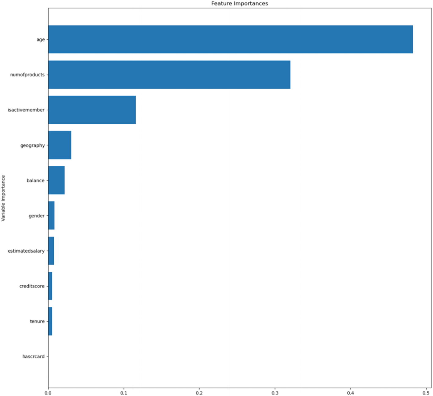
Automated model feature importances

../images/500182_1_En_8_Chapter/500182_1_En_8_Fig14_HTML.jpg
Figure 8-14

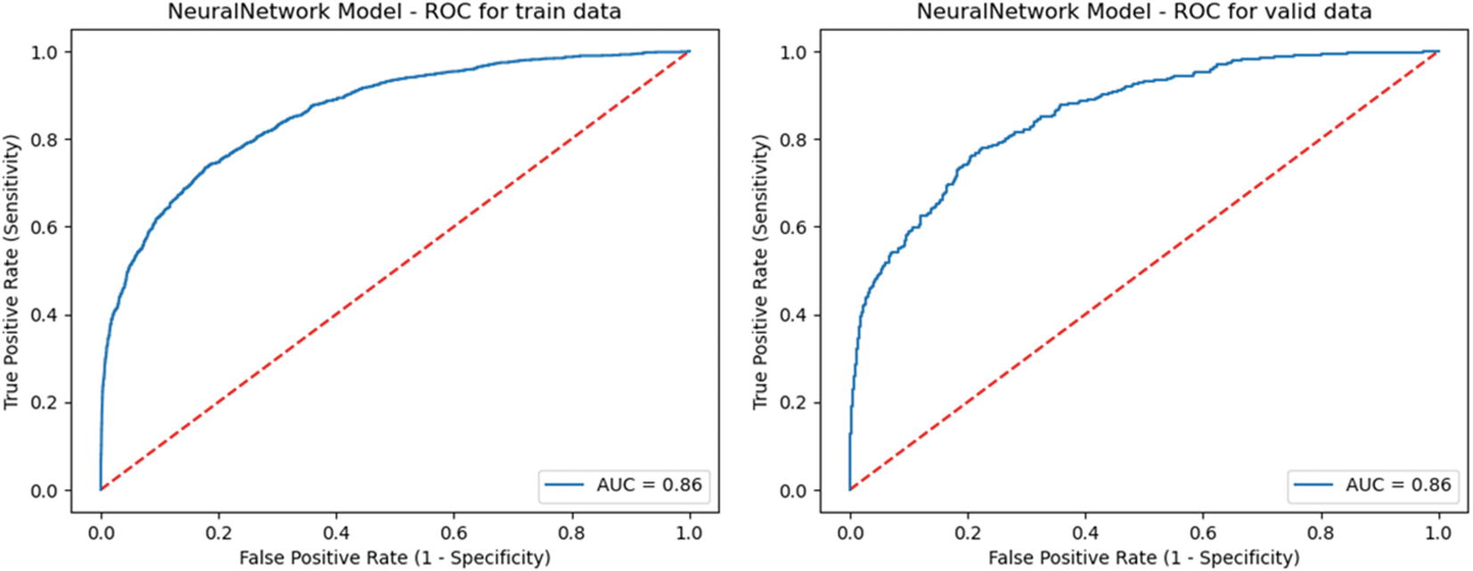
Automated model ROCs

../images/500182_1_En_8_Chapter/500182_1_En_8_Fig15_HTML.jpg
Figure 8-15

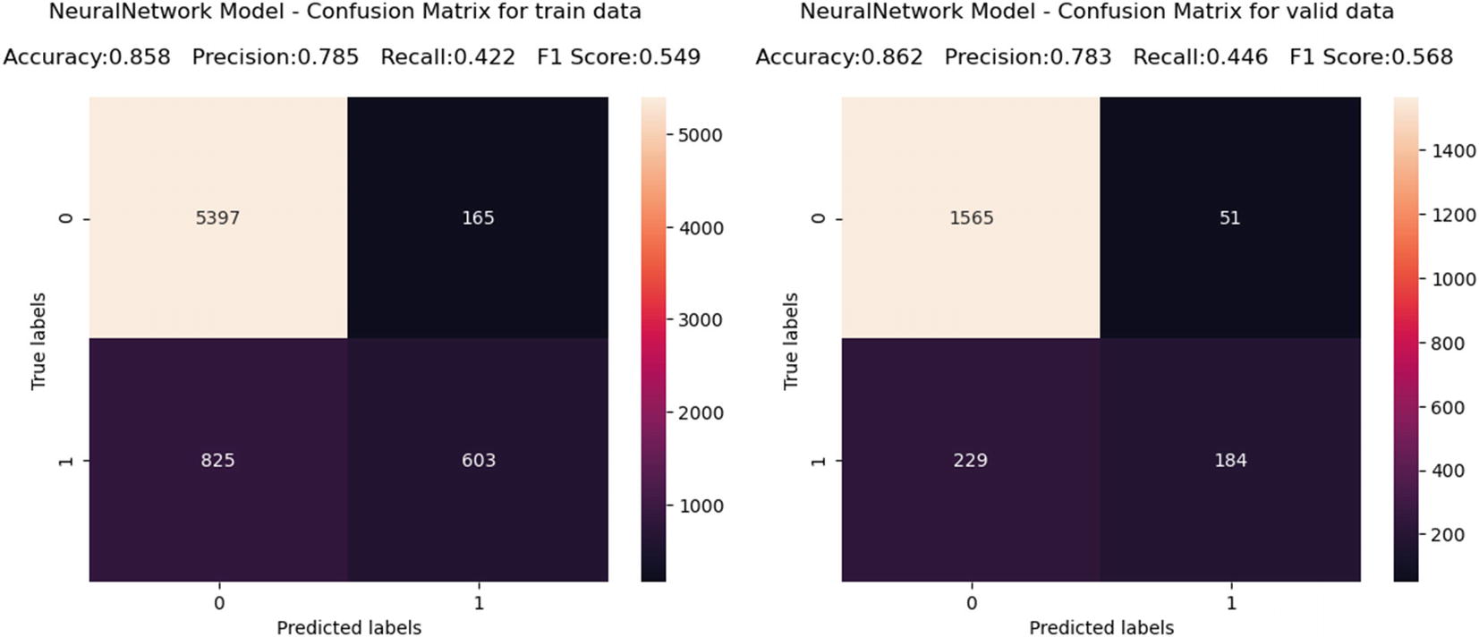
Automated model — Confusion matrix

Table 8-4

Combined Metrics

model_type

roc_train

accuracy_train

ks_train

roc_valid

accuracy_valid

ks_valid

neuralNetwork

0.86171092

0.858369099

55.5

0.857589

0.862000986

54.43

randomForest

0.838162018

0.860228898

50.57

0.835679

0.856086742

50.48

logistic

0.755744261

0.81230329

37.19

0.754326

0.807294234

37.31

gradientBoosting

0.881999528

0.869384835

59.46

0.858617

0.853622474

55.95

model_type

roc_test

accuracy_test

ks_test

roc_oot1

accuracy_oot1

neuralNetwork

0.813792

0.849134

46.58

0.856175

0.8582

randomForest

0.806239

0.840979

44.3

0.834677

0.8575

logistic

0.719284

0.805301

32.19

0.751941

0.8106

gradientBoosting

0.816005

0.850153

47.22

0.870804

0.8643

model_type

ks_oot1

roc_oot2

accuracy_oot2

ks_oot2

selected_model

neuralNetwork

54.43

0.856175108

0.8582

54.43

Champion

randomForest

49.99

0.834676561

0.8575

49.99

Challenger

logistic

36.49

0.751941185

0.8106

36.49


gradientBoosting

57.51

0.870803793

0.8643

57.51

 
Table 8-5

Kolmogorov-Smirnov Statistic

-../images/500182_1_En_8_Chapter/500182_1_En_8_Figa_HTML.jpg

Table 8-6

Neural Network Test

-../images/500182_1_En_8_Chapter/500182_1_En_8_Figb_HTML.jpg

This module is intended to help you create quick, automated experiments and is in no way meant to replace the model-building activity.

EXERCISE 8-2: BUILDING CUSTOM PIPELINES

Question: We challenge you to build a separate pipeline or integrate code flow to accommodate continuous targets.

Summary

  • We learned the challenges of model management and deployment.

  • We now know how to use MLflow for managing experiments and deploying models.

  • We explored how to build custom pipelines for various model-building activities.

  • We saw how pipelines can be stacked together to create an automated pipeline.

Great job! You are now familiar with some of the key concepts that will be useful in putting a model into production. This should give you a fair idea of how you want to manage a model lifecycle as you are building your data-preparation pipelines. In the next chapter, we will cover some of the tips, tricks, and interesting topics that can be useful in your day-to-day work.

..................Content has been hidden....................

You can't read the all page of ebook, please click here login for view all page.
Reset
3.17.150.89