3
Linear Elements and Networks
3.1 The Linear Features and Corridors in the Landscape
Linear features in the landscape are commonly created both by nature, such as streams, ridges, and animal trails, or by humans, such as roads, powerlines, ditches, and walking trails1. These linear features affect many ecological characteristics and processes in a landscape, including the influence of wind, solar radiation, the movement of disturbances, or the movement of organisms.
One can consider two categories of linear features: line corridors and strip corridors. Both types of linear features may have the functions of conduits (corridors), barriers or filters for the movement of organisms, disturbances, or for the flow of water, soil, or nutrients. However, strip corridors differ from line corridors in that their width is important for the process or organism of interest, as when they are sufficiently wide to provide habitat and also functions in the landscape, acting as a source or sink for organisms, matter, or disturbances.
Since the difference between line corridors and strip corridors is whether or not they provide habitat (and therefore possible source or sink functions), the distinction is often only a matter of scale and the objective of the analysis.
Literature about corridors is abundant and rapidly increasing. It typically concentrates on riparian vegetation, hedgerows, and roads, but studies have also considered how railroads, dikes, ditches, fences, powerlines, and vegetation strips influence wildlife movements.
There are many references on such studies from the very beginning of landscape ecology. The study on the ecological effects of roads have been developing in many countries2, especially after Forman published the very influential book reviewing our knowledge on the effects of roads on organisms and processes at the landscape level in what was referred to as “road ecology”3.
Many of the studies on corridors are dedicated to their function as conduits for organisms, for the dispersal of plant seeds, and for the movement of animals by facilitating the movement through otherwise unsuitable habitat. They may also act as transportation or recreation pathways for humans (Figure 3.1).

Figure 3.1 Ecological functions of line (and strip) corridors, which may act as conduits, barriers, or filters (top row). In addition, strip corridors (bottom) may also act as habitat, sources, or sinks.
(adapted from Smith, D.S. and Hellmund, P.C. (1993) Ecology of Greenways: Design and Function of Linear Conservation Areas, University of Minnesota Press, Minneapolis, MN)
In contrast, corridors may also serve as barriers to organism movements, including humans, depending on the characteristics of the corridor and the requirements of the organism in question. The filtering function of corridors can be likened to acting as a leaky barrier that restricts the movements of some organisms but not others. This filtering function is not limited to organisms. In riparian zones along stream corridors, eroded soil can be trapped and chemicals can be filtered out of soil water by plant roots and soil microbes. They may also act as a filter to disturbances. For example, fire may cross a strip under some types of weather conditions but not others.
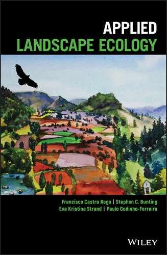
Greenways are special types of corridors that are implemented in or near urban environments and function primarily as a conduit for humans with a focus on recreation and aesthetics4, but that may also provide many other ecological functions (Figure 3.2).
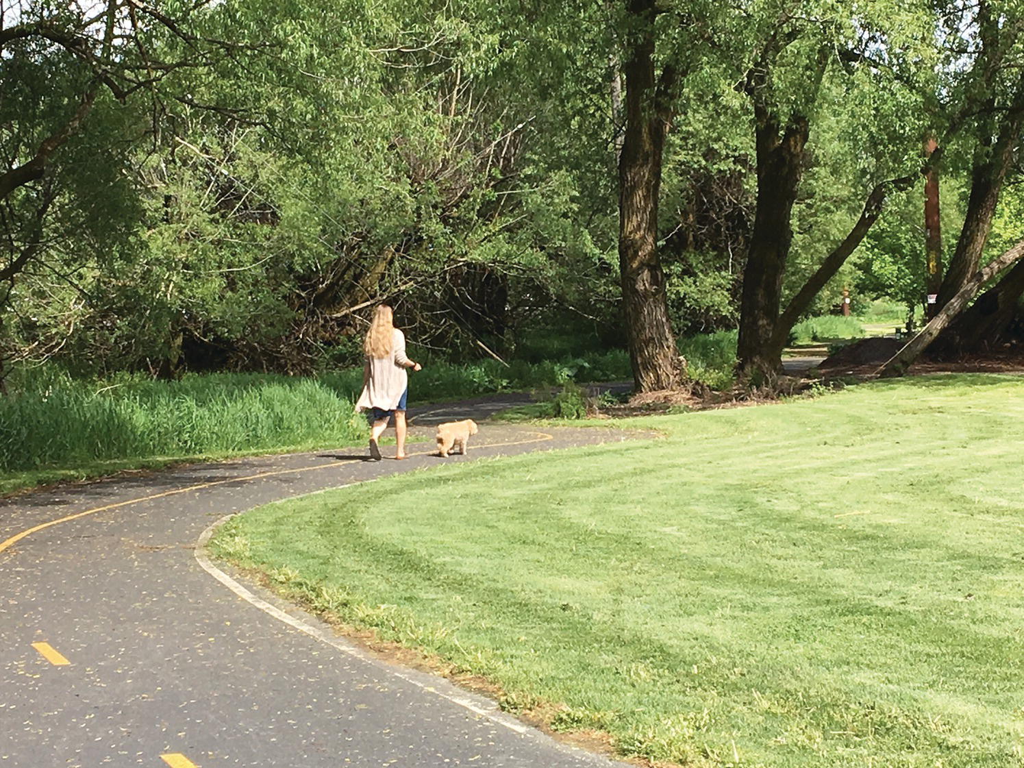
Figure 3.2 Greenway in Moscow, Idaho, USA. Photo by Stephen Bunting.
Various types of greenways were already described in 1990 by Charles Little in his fundamental book Greenways for America: “a linear open space established along either a natural corridor, such as a riverfront, stream valley, or ridgeline, or overland along a railroad right‐of‐way converted to recreational use, a canal, scenic road or other route; a natural or landscaped course for pedestrian or bicycle passage; an open‐space connector linking parks, nature reserves, cultural features, or historic sites with each other and with populated areas; locally certain strip or linear parks designated as parkway or greenbelt”5.
Possibly the first clear example of a greenway was that created in 1880 by Frederick Law Olmsted in his “Emerald Necklace” plan for the Boston Park System (Figure 3.3).
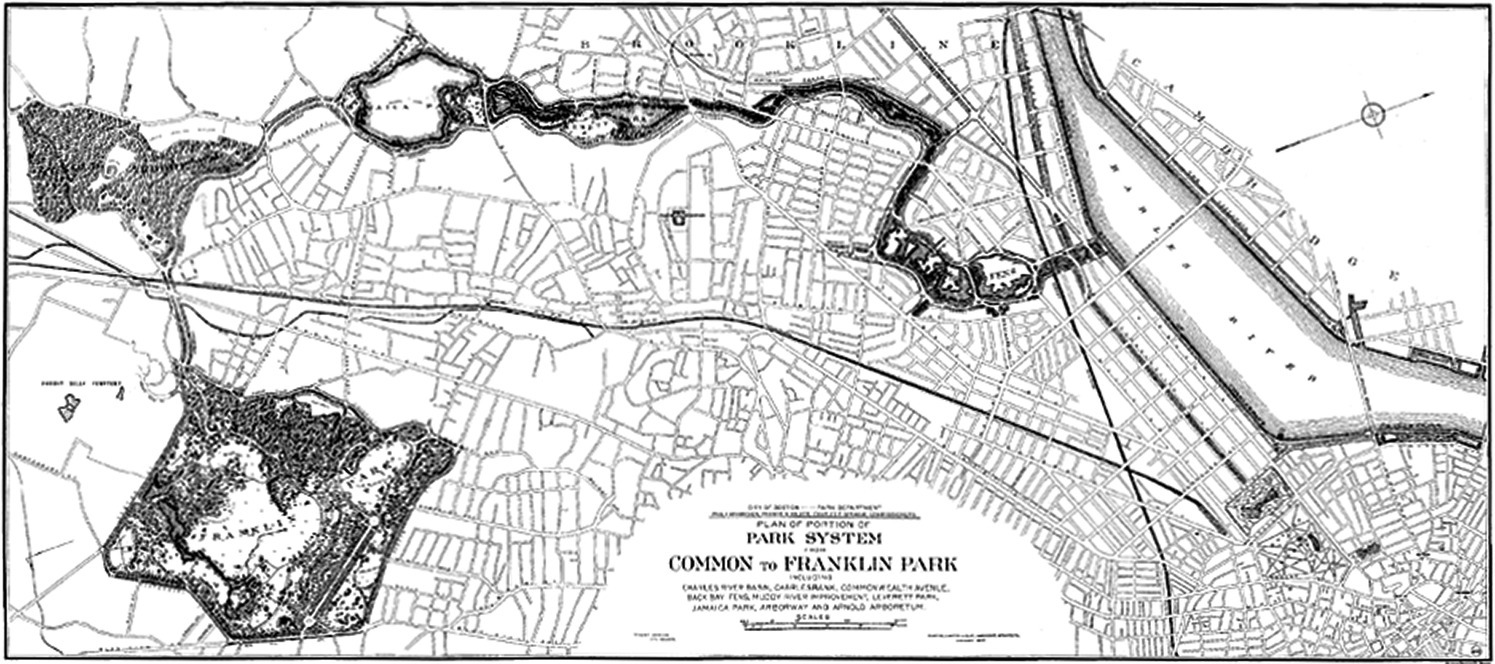
Figure 3.3 The Olmsted Plan “Emerald Necklace”, a greenway in the urban area of Boston.
The modern study of the ecology of greenways6 began in 1993 but, since the very beginning, the word “greenways” has been used with many different meanings. However, in spite of some confusion around its definition, the concept gained popularity and appeared regularly in popular language and planning policy in the USA. An international movement was then beginning, as announced by Julius Fabos and Jack Ahern in 19967. A good review of the use of greenways for strategic landscape planning was provided by Ahern in 20028.
The linear features in the landscape, whatever their function and context will be, need to be characterized in order to make it possible to understand their relationships with landscape processes.
3.2 Curvilinearity and Fractal Analysis
We will start the analysis of linear elements by the simple case of one single line (no width). This seems simple in that the only characteristic that is generally quantified is the length. Of course, length is a very relevant measurement with very important ecological consequences. The length of a river, for instance, determines the amount of adjacent riparian vegetation. The length of a road determines the number of houses that can be built adjacent to it if the distance between them is fixed. The length of a coastal line also determines the amount of habitat coastal nesting birds have to utilize.
However, the measurement of the length is not as simple as it seems. The “length” of a coastline was considered to be a very difficult characteristic and not a meaningful measure in many studies, such as that of Pennycuick and Kline9 when they studied the distribution of bald eagle nests in the cliffs of the coasts of the Aleutian Islands of Alaska (Figures 3.4 and 3.5).

Figure 3.4 Maps of Adak and Amchitka Islands in Alaska, USA. The arrows point to bald eagle (Haliaeetus leucocephalus) nest sites.
Source: Pennycuick, C.J. and Kline, N.C. (1986) Units of measurement for fractal extent, applied to the coastal distribution of bald eagle nests in the Aleutian Islands, Alaska. Oecologia, 68, 254–258.

Figure 3.5 Bald eagle (Haliaeetus leucocephalus) in its nest in the coastal habitat.
Source: http://www.arkive.org/bald‐eagle/haliaeetus‐leucocephalus/image‐G54270.html; http://cdn1.arkive.org/media/67/678A6C5F‐678B‐4B13‐8711‐3171264AF87E/Presentation.Large/Bald‐eagle‐in‐nest‐in‐coastal‐habitat‐.jpg.
In fact, most attempts to measure density of organisms that are distributed along irregular boundaries, such as coastlines, have the fundamental difficulties associated with the unit of measurement. Therefore we need, again, to look at the scale appropriate to the organism or the process of interest.
A common example illustrating the importance of scale and the measurement unit is the estimation of the length of the coast of Britain (Figure 3.6). Here, again, the coastline is difficult to define. In order to answer the question we have to realize that the response depends on how closely you look at it or how long your measuring ruler is. The answer is that the length of the coastline seems to get longer and longer as you measure it more closely.
Figure 3.6 Land’s End, at the tip of Cornwall, Great Britain.
We can now use the concept of fractal dimension to describe the coastline, as did Mandelbrot (Figure 3.7) in 1967 is his very influential article on fractals on “how long is the coast of Britain?”10.

Figure 3.7 Benoit Mandelbrot (1924–2010), the pioneer of fractal geometry.
In order to see how the measured length changes with scale we need to measure the coastline using rulers as segments of different lengths, as if we were considering different species of territorial birds that would require different distances between nests.
Let us define the length of the ruler as a segment of size s and that we measure the coastline as the number of segments (n) (Figure 3.8).
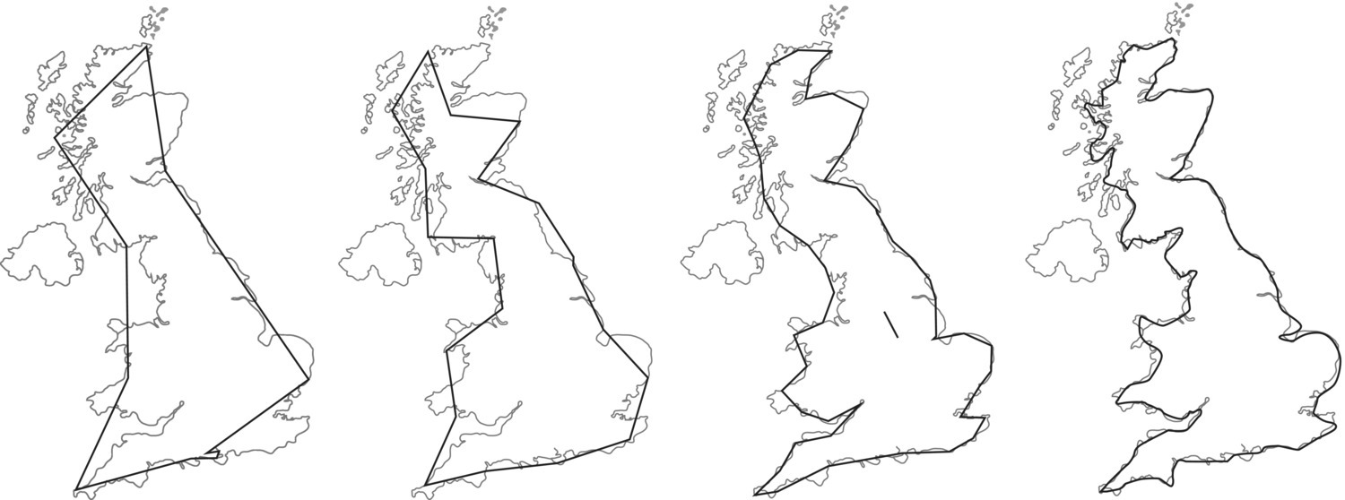
Figure 3.8 Measurements of the coastline of Great Britain using different ruler lengths, varying from 400 km, 200 km, 100 km, and 50 km, from left to right.
With a larger ruler (the first image to the left) the segment size is s = 400 km, the measured number of segments is n = 9, and the estimated length is therefore ns = 3600 km. For the 200 km ruler the number of segments is 19 and ns = 3800 km, for the 100 km ruler n = 48 and ns = 4800 km, and for the smaller ruler (s = 50 km) the measured number of segments is n = 97 and the estimated length of the coastline is ns = 4850 km.
With a perfectly linear coastline the estimated lengths should be similar (L) and therefore ns = L or n = L/s. For the more general case, however, we have
where L is a constant (the length of a reference line), s is the size of the ruler, and D is termed the fractal dimension of the line, which is a measure of its curvilinearity. If the line is not curvilinear (a straight line) the value of D will be unity and we will have the simple case where n = L/s. The closer to one the dimension D is, the straighter and smoother the coastline is. The higher the dimension (the closer to two) is, the more jagged and wiggly the coastline is11.
If we take the natural logarithm of the measured values we can fit a straight line of the form:
In this case the fractal dimension of the coastline, D, is simply the slope of the line.
It is easier to see this relationship in a graph where the number of segments needed to measure the coast of Britain (shown in Figure 3.8) is plotted against the size of the ruler used (Figure 3.9).
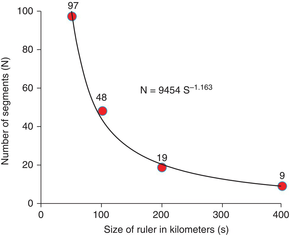
Figure 3.9 Relationship between the number of segments needed for the measurement of the coast of Britain and the size of the ruler used (in kilometers). The power equation fitted is shown, indicating that the fractal dimension (D) is equal to 1.163.
We can also fit a power equation to the relation between n and s and find that the exponent is approximately D = 1.163, which is our estimate of the fractal dimension of the coastline of Britain.
The final equation for the length of the coastline measured in number of segments is
and the estimated length ns is therefore
The value of k (9454 km) is the estimate of the length of the coast measured with a 1 km ruler. As the exponent of s is negative, this equation shows that the estimated length of the coastline decreases with the increasing size of the ruler (s). If the coastline was a straight line the value of D would be 1 and the measured length would always be L independently of the size of the ruler.
We can now use this equation to estimate how many objects there could be along the coastline knowing the required distance from each other (s). Scale is now included in the solution. The length of the coastline depends upon the ruler used to measure it and the ruler depends on the organism of interest (distance between bald eagle nests, for example).
Similarly to what was done for points in the previous chapter, we can apply methods that use distances (as rulers in this case) or quadrats. In this latter case we can use the box counting method, which is analogous to the length measuring method previously used (Figure 3.10). We start by using a large grid (400 km side) and count the number of boxes (quadrats) of the grid where the coastline is included. Then we repeat the measurement using successively smaller boxes.
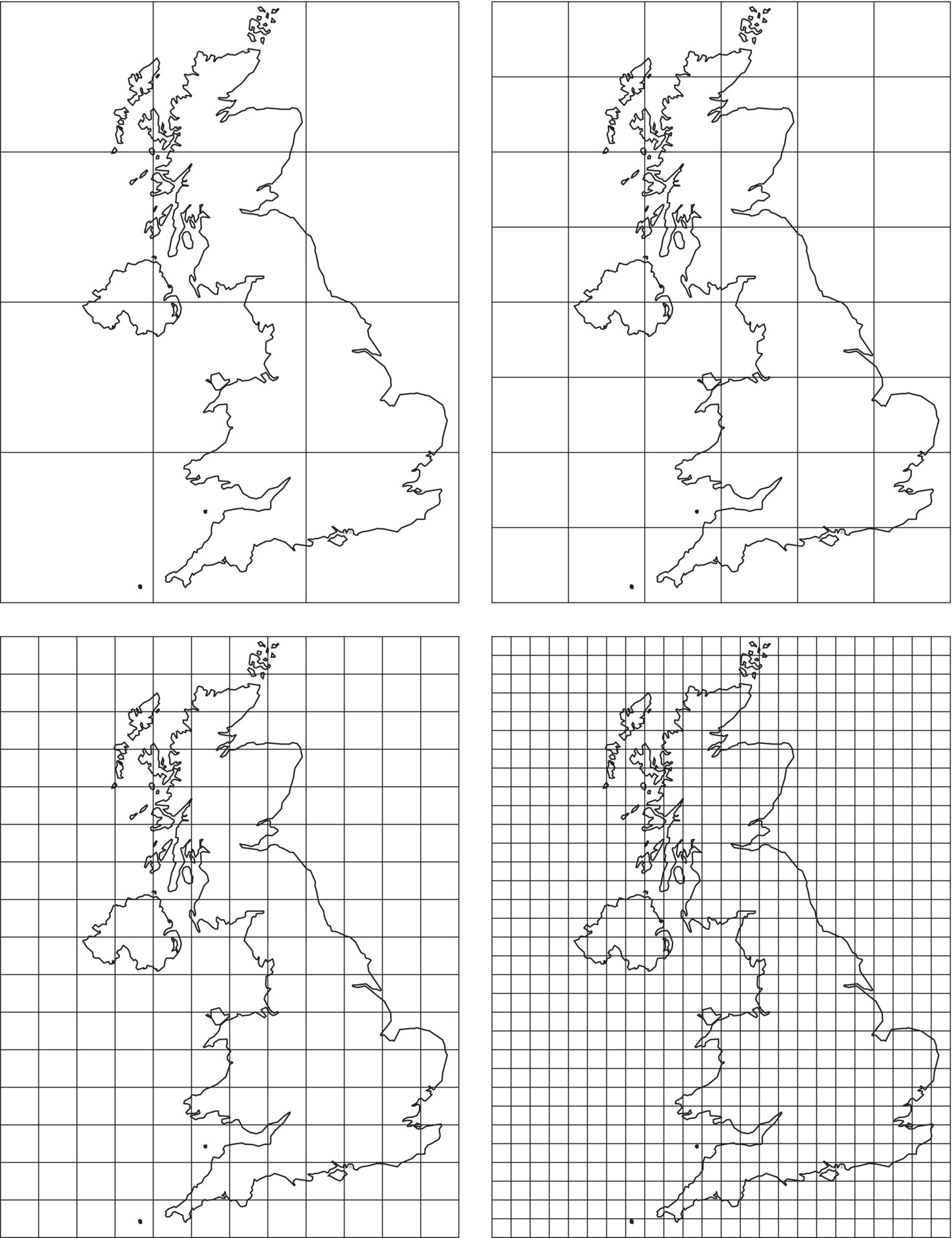
Figure 3.10 The box counting method applied to the coastline of Britain.
Similarly to what was done with the ruler, we can now plot n against s, where s is now the side of the box, as shown in Figure 3.11.
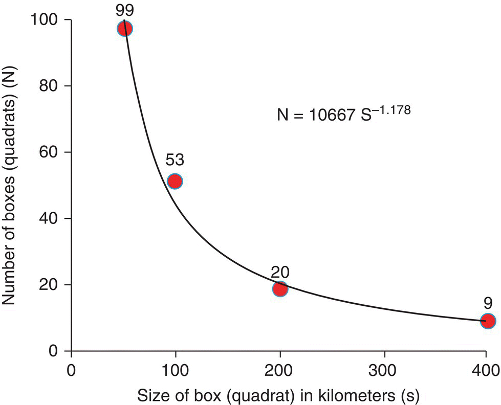
Figure 3.11 The best fit for a power equation for the results of the box counting method for the coastline of Britain. The estimate of the fractal dimension of the coastline of Great Britain is therefore D = 1.178.
The results of both methods indicate similar values for the slope (D = 1.163 and D = 1.178, respectively). The distance (ruler) and quadrat (box counting) methods are equivalent in determining the fractal dimension of lines, that is, their curvilinearity.
Rivers, when reduced to lines, indicate the same effects of measurement scale as coastlines (Figure 3.12). The shape of the river has important consequences on hydraulic and biotic processes. Greater curvilinearity usually results in a decreased stream gradient, which influences the erosion power and potential sediment load capacity of a river. Sinuous streams have a greater riparian habitat and often more diversity in the types of habitat. Curvilinearity may also influence stream characteristics such as temperature, oxygen content, and productivity.
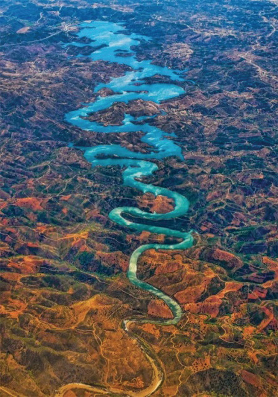
Figure 3.12 Image of strong curvilinearity of a river close to Faro, Portugal.
Source: Image courtesy of REDDIT user Docious.
The concept of a fractal dimension can be used to describe the complexity of all shapes. From this example we understand that as a line changes from straight to a more irregular shape the fractal dimension D changes from 1 and approaches the value of 2 as the line fills the whole area. Using the same concept we can include a third dimension and as the irregularity of the surface increases the fractal dimension D increases from 2 and approaches the value of 3 as the surface fills the whole volume. Likewise, as a straight line is fragmented, the fractal dimension D approaches 0. The value of 0 is the fractal dimension of a point. This is illustrated in Figure 3.13.
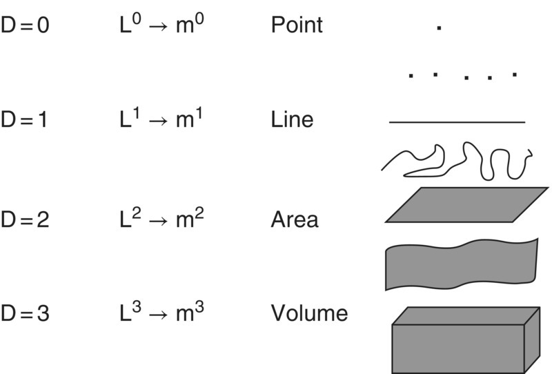
Figure 3.13 Representation of shapes from the more simple (a point with fractal dimension D = 0, nondimensional) to the more complete (a volume with fractal dimension D = 3, with units of length L 3, commonly measured in cubic meters, m3).
3.3 Linear Density of Networks
We will now consider a network of lines. Of course, individual lines can be quantified by the method presented earlier. However, there are several attributes that can be used specifically to describe a network of linear elements in a landscape.
The most important single characteristic is the line (or corridor) density, as a measure of the abundance of corridors in an area, which can be simply defined as the total length of linear elements per unit area. The line density (λl) is given by
where li is the length of line i and TL is the total length of lines within the area TA.
For watersheds this concept is used in defining drainage density as the total length of streams divided by the area of the drainage basin. Drainage density is often reported in units of km/km2 or km−1 and values from less than 2 km−1 to over 100 km−1 have been reported as a function of climate, soils (less permeable soils result in more surface water runoff and higher drainage density values), and topography (watersheds with steep slopes tend to have a higher drainage density).
It can be shown that the average distance from the basin divide to a stream is 1/(2λl) and that the average distance that a drop of water from a rainfall event travels to a stream is also inversely proportional to the drainage density. Watersheds with a high drainage density have a shorter response time to a precipitation event and a sharper peak discharge. Thus, drainage density is an indicator of the efficiency of the stream network in the process of draining an area and it has been used in the predictions of the magnitudes of flood flows or low flows (Figure 3.14)12.
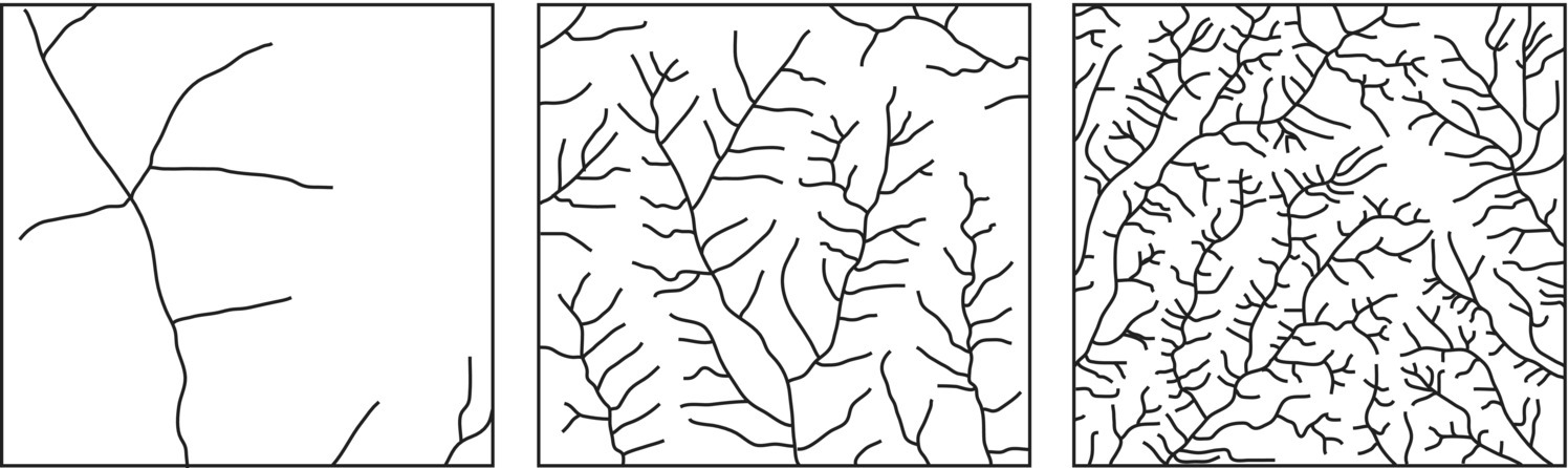
Figure 3.14 Areas with different drainage densities, increasing from left to right.
Source: fao.org (Food and Agricultural Organization of the United Nations).
Drainage density applies for the length of the streams, but the concept of linear density can also apply to any other network of lines on a map. We can also define the linear density of ridges and of contour lines. In watershed studies the density of contour lines is directly related to the average slope of the watershed. However, the density of contour lines has also been used to estimate landscape ruggedness relevant for many different processes, such as for the “escape terrain” for bighorn sheep (Orvis canadensis)13,14 (Figure 3.15).
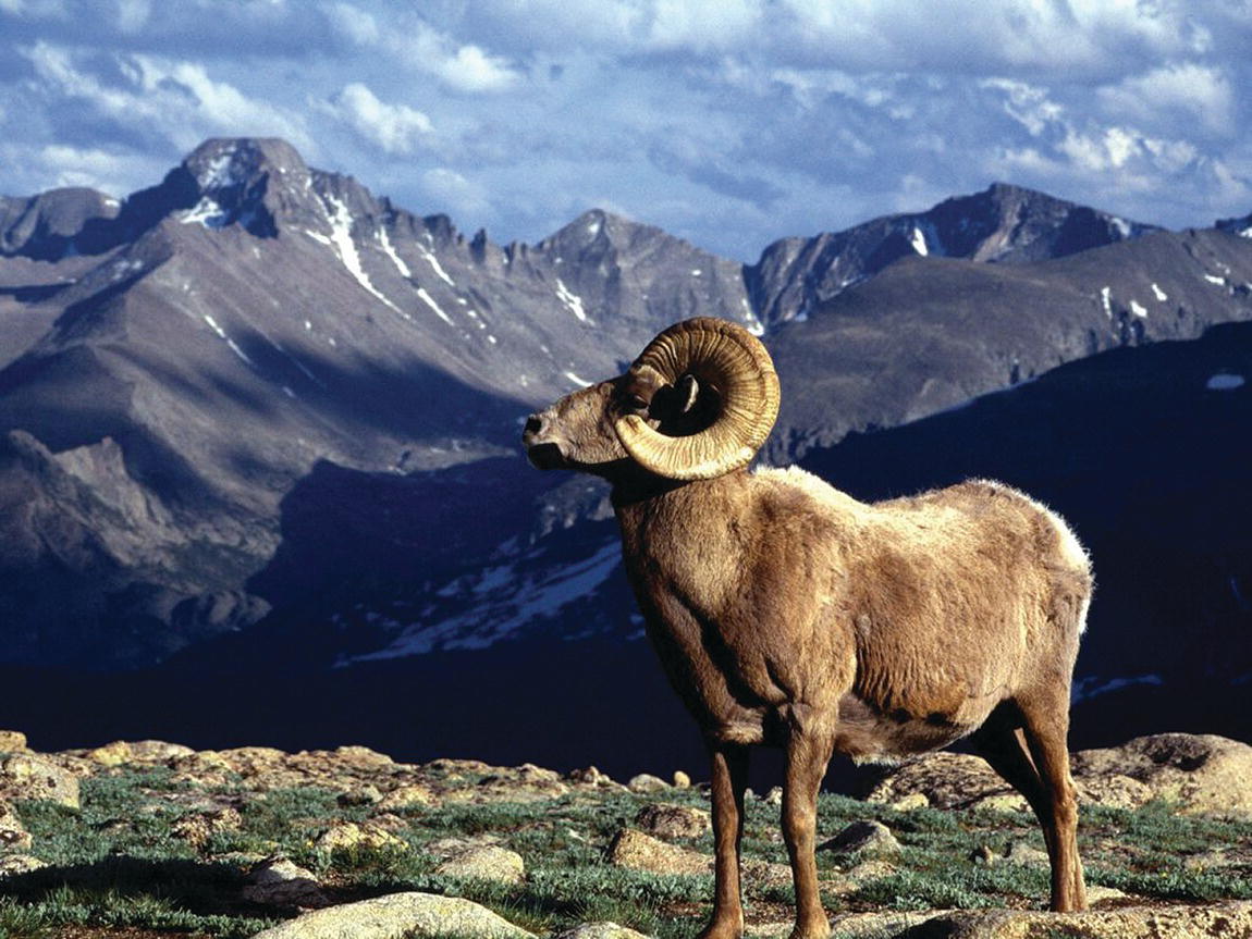
Figure 3.15 Bighorn sheep (Ovis canadensis) in rugged terrain.
The effects of linear networks in ecological processes are many and are dependent on the type of network and the process considered. One such cause–effect relationship that has been abundantly reported in the literature is the effect of road density, a linear network, in inhibiting movement of large wildlife species. These results have been used to close some roads and to propose specific forest management schemes in order to mitigate the impact of road networks on sensitive wildlife species15.
Some wildlife species have been shown to be particularly affected by road density. Sensitivity to road density has been demonstrated in a study on grizzly bears (Ursus arctos horribilis) in Idaho, concluding that open roads greatly influenced the distribution of bears (Figure 3.16). Areas with high open road density (>2.6 km−1) were avoided or used much less than expected if the landscape had been randomly used16.
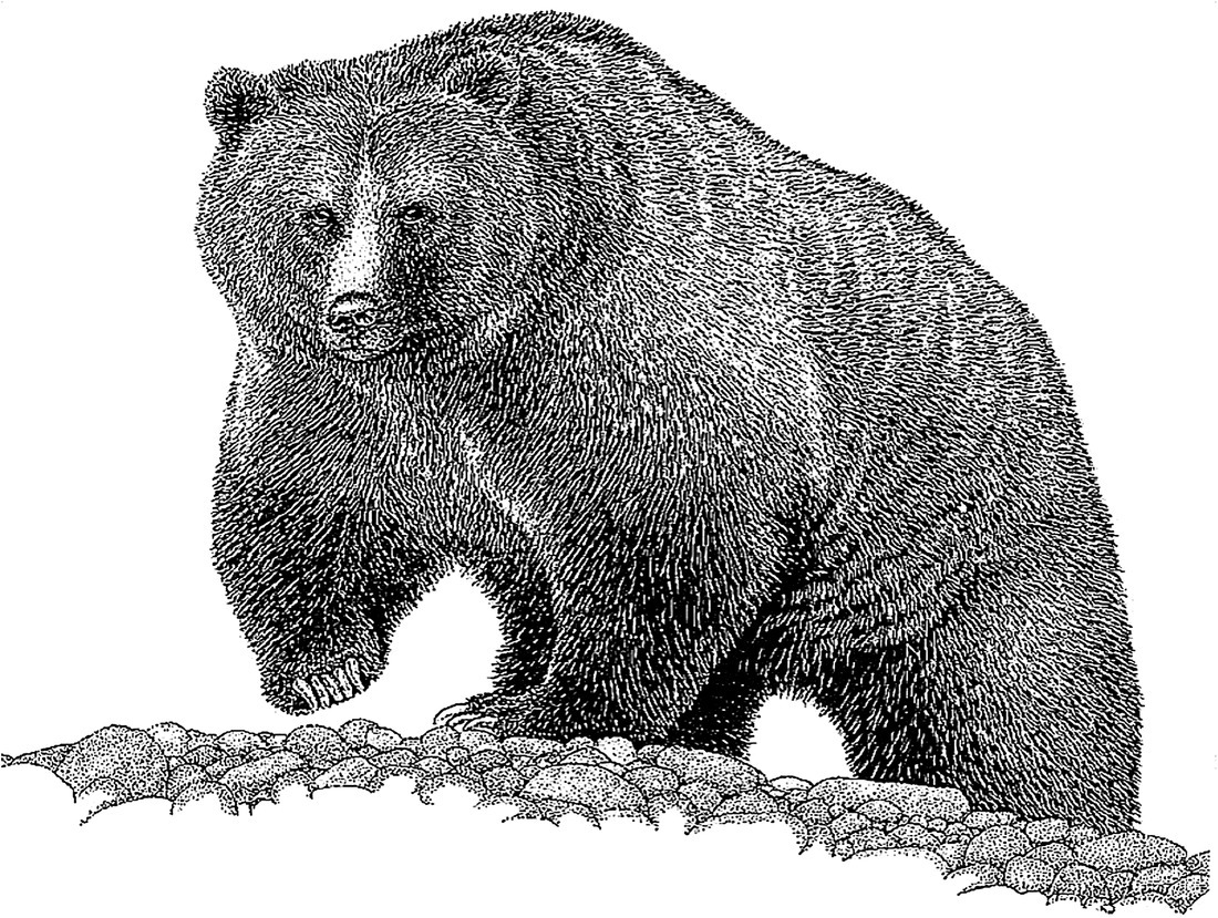
Figure 3.16 Grizzly bear (Ursus arctos horribilis) image from the report of the study in Idaho17.
Similar studies were conducted in other regions. Recent research has shown the negative impact of road density on survival rate of grizzly bear populations in Alberta, Canada (Figure 3.17)18.

Figure 3.17 The negative relationship between road density (km−1) and survival rate of subadult males and females in a study of grizzly bear in Alberta, Canada.
Source: Boulanger J. and Stenhouse, G.B. (2014) The impact of roads on the demography of grizzly bears in Alberta. Open‐access article. PLoS ONE, 9 (12), e115535.
3.4 Spatial Distribution of Linear Networks
Apart from linear density, linear networks can also be described by their spatial distribution, as they are also known to affect landscape processes on many scales. We could use quadrat methods in exactly the same way that they were used for points. In that case a fractal dimension for the network of lines can be determined exactly as if it was a single line. However, the quantification of the spatial distribution of lines is less well developed and used than those applied to the pattern of points. One of the most common methods to examine the distribution of distances between lines is by calculating nearest‐neighbor distances19.
The steps required for this technique include:
- Randomly pick a point on one of the lines (i) in the landscape.
- From that point in line (i), measure the distance to the nearest line in a direction perpendicular to the line (di), as shown in Figure 3.18.
- Randomly pick other points on other lines and repeat the procedure.
- Compute the observed mean nearest‐neighbor distance (OMD) for the n distances measured:

- Compute the expected mean nearest‐neighbor distance (EMD) for a pattern of random lines with the equation20
where λl is the line density.

- Compute a nearest‐neighbor index (PATTERN2) identical to that used for point patterns by taking the ratio

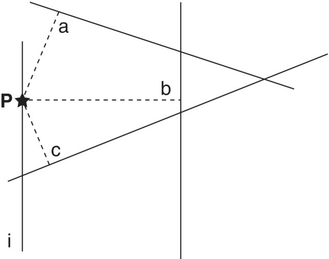
Figure 3.18 The distance of the random point P in line i to the nearest line is di = c.
Similarly to what was indicated for point distribution, the meaning of the index is
The calculations are illustrated in Figure 3.19.
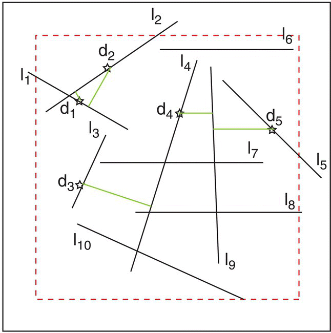
Figure 3.19 Distribution of lines used for the exercise, where li is the length of line i and di is the nearest‐neighbor distance from a point on line i.
If the total length of these lines (TL) is 43 km and the area (TA) is 100 km2 the linear density is calculated as
If the n = 5 distances measured (km) inside the inner area (to avoid edge effects) were d1 = 0.2, d2 = 1.2, d3 = 2.1, d4 = 1.0, and d5 = 1.8, we would compute the observed mean nearest‐neighbor distance (OMD) as
We can now compute the expected mean nearest‐neighbor distance (EMD in the hypothesis of a random distribution) as
and the ratio PATTERN2 can now be calculated as
As the value of PATTERN2 is well above unity (PATTERN2 > 1) we can conclude that the distribution of lines tends to be clustered.
An alternative system to detect patterns in the distribution of lines is by constructing a number of auxiliary transect lines over the region of interest, counting the number of times these auxiliary lines cross the lines of the network, and measuring the distance between those lines (di) (Figure 3.20).

Figure 3.20 Distribution of lines used for the exercise, where li is the length of line i and dj is the distance between lines.
The same example would indicate that the measured distances (km) are now d1, d2, d3, d4, and d5. The variance of these distances is also a good measure of departure from absolute regularity when the variance is zero.
The relationships between the total number of crossings (CROSS) and the total length of the auxiliary lines (TLA) is also very important since it allows for the estimation of linear density by λl = π CROSS/(2 TLA). In this case, with 5 crossings (CROSS = 5) and a total length of the two auxiliary lines TLA = 20 km, we would estimate the linear density to be 0.39 km−1, close to the measured value of 0.43 km−1. These relationships were established and used successfully for stream networks21. These methods work well for lines that do not frequently reverse directions and that are at least 1.5 times longer than the average distance between lines22.
This method of using auxiliary transect lines is extremely useful as it can provide information simultaneously about linear density and distribution.
3.5 Analysis of the Spatial Distribution of Linear Networks
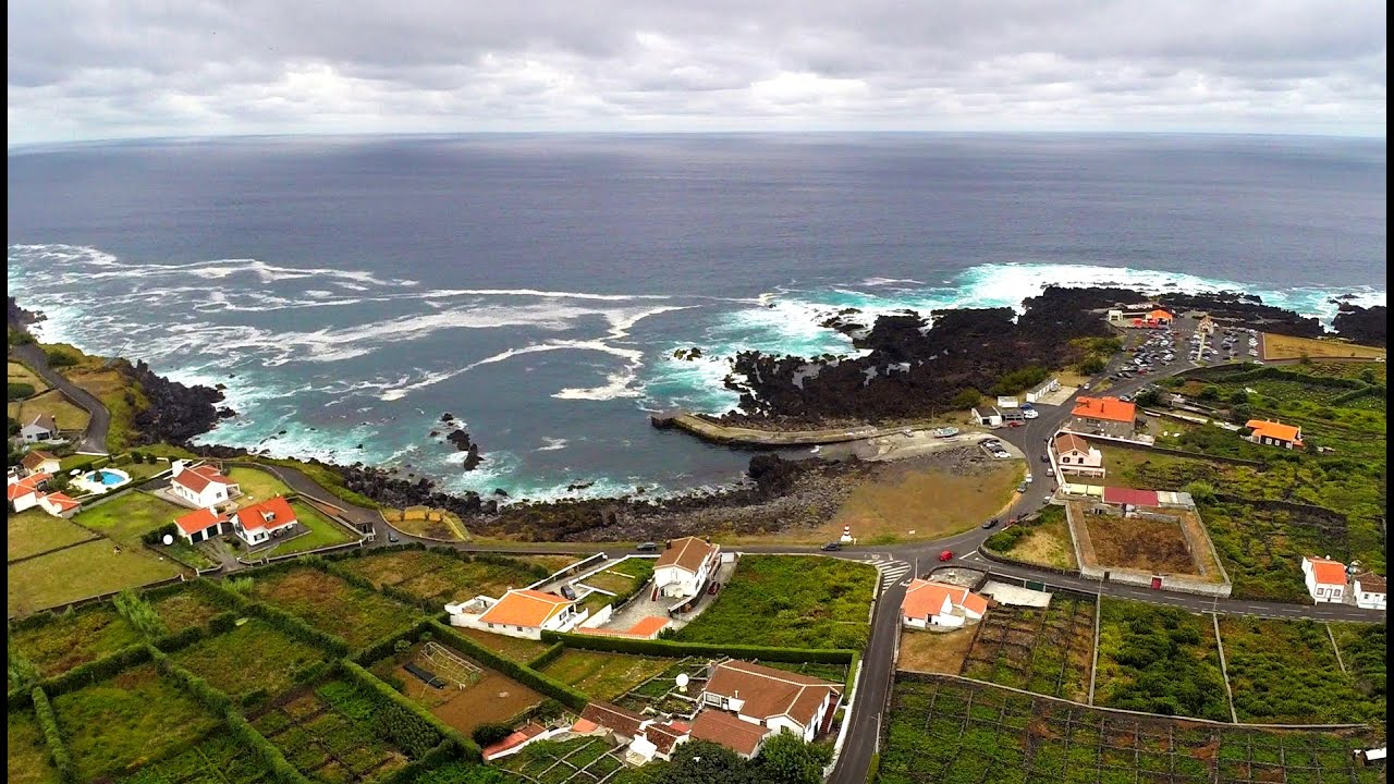
To illustrate the process fully we can use a worked example from the northern coast of the island of Terceira, Azores, where the traditional agricultural fields are separated by stone walls (from lava flows) or hedgerows with woody species such as the firetree (Myrica faya) (Figure 3.21).
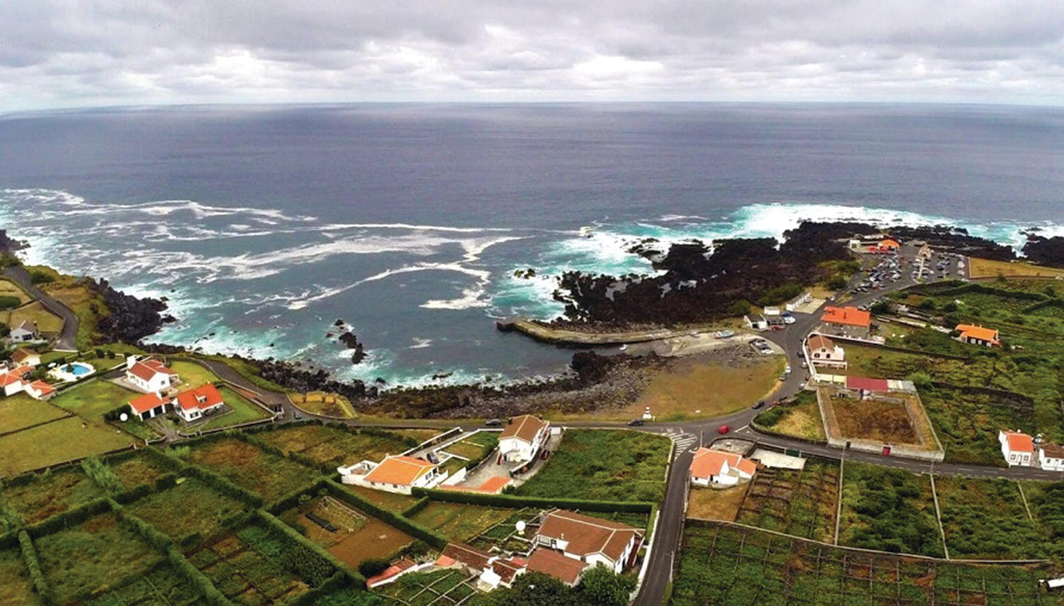
Figure 3.21 A view of the area of Biscoitos, on the island of Terceira, Azores, showing the stone walls and the hedgerows separating the small agricultural fields.
Source: Manuel Cunha, SKai aerial image, http://i.ytimg.com/vi/BLh2d8qFzYM/maxresdefault.jpg.
We can now analyse the pattern of the lines that separate the agricultural fields using the images of the same general region from Google Earth (Figure 3.22).

Figure 3.22 A view of the northern coast of the island of Terceira, Azores, close to Biscoitos. We used four auxiliary transect lines divided into 112 segments of 50 m (upper image) and 56 segments of 100 m (lower image).
Source: Google Earth.
In a way similar to what was done for point counts in quadrats, we can now count the number of crossings between the segments in the transect lines and the edges of the fields. A summary of the results obtained and the calculations of the mean and variance are presented in Tables 3.1, 3.2, and 3.3.
Table 3.1 A summary of the crossings of the transects with 100 m segments.
| Number of crossings per segment (x) | Number of segments (nx) | (nx)(x) | (nx)(x – MEAN)2 |
| 0 | 1 | 0 | 3.5 |
| 1 | 17 | 17 | 12.6 |
| 2 | 28 | 56 | 0.5 |
| 3 | 9 | 27 | 11.7 |
| 4 | 1 | 4 | 4.6 |
With:
Table 3.2 A summary of the crossings of the transects with 50 m segments.
| Number of crossings per segment (x) | Number of segments (nx) | (nx)(x) | (nx)(x – MEAN)2 |
| 0 | 25 | 0 | 21.6 |
| 1 | 71 | 71 | 0.3 |
| 2 | 15 | 30 | 17.2 |
| 3 | 1 | 3 | 4.3 |
With:
Table 3.3 Summary of the counts of crossings per segment.
| Segment size (s) | MEAN of the number of crossings | VARIANCE of the number of crossings | VARIANCE/MEAN ratio (VMR) |
| 100 | 1.86 | 0.59 | 0.32 |
| 50 | 0.93 | 0.39 | 0.42 |
As the variance to mean ratio (VMR) is well below unity, we conclude that the lines (the limits of the agricultural fields) were regularly distributed at both scales (100 m and 50 m).
As for points, we could now calculate the expected number of segments under the null hypothesis of a random (Poisson) distribution with the same mean values, and test that hypothesis with a chi‐square test comparing observed and expected counts.
Finally, by knowing that there is a relationship between the total number of crossings (CROSS) and the linear density (λl) of the form:
where TLA is the total length of the auxiliary transect lines (TLA = 5.6 km), we have
These calculations show that the method of the auxiliary transect lines can be very useful to provide information for both linear density and distribution pattern, two very important characteristics of the distribution of linear features in the landscape.
3.6 A Study of Linear Features on the European Scale
A good example of a study that used these methods was that of van der Zanden and others23 who used 250 m line transects in a sampling grid throughout Europe and recorded the number of crossings with linear features (Figures 3.23 and 3.24).
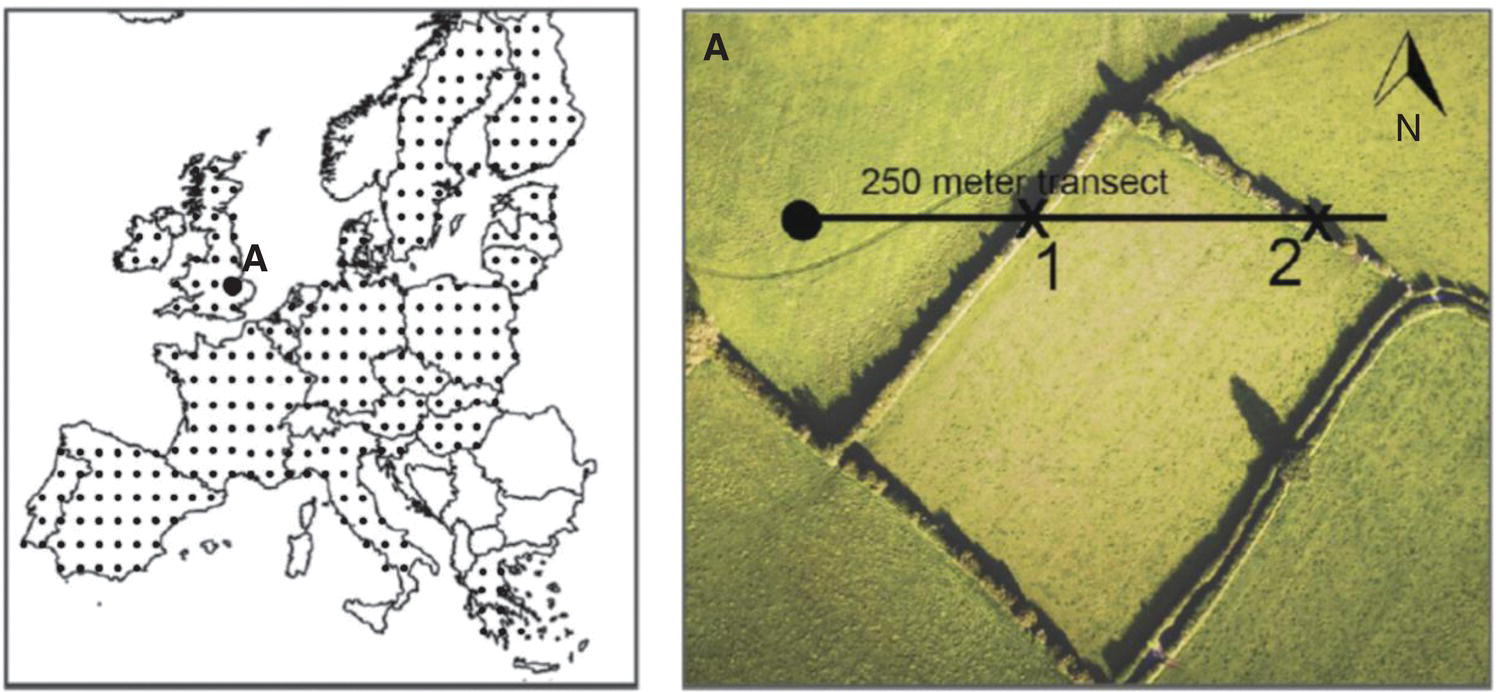
Figure 3.23 An overview of the grid used in transect‐sampling linear features in Europe, with an example from southeastern Britain.
Source: Van derZanden, E.H., Verburg, P.H., and Mucher, C.A. (2013) Modelling the spatial distribution of linear landscape elements in Europe. Ecological Indicators, 27, 125–136.

Figure 3.24 Results of the study showing the frequency of counts per transect for the three different types of linear features analyzed: green lines (hedge and tree lines), ditches, and grass margins (left). On the right, the spatial model of the results for hedge and tree lines showing higher densities in some regions where they are part of traditional agricultural landscapes in France, England, Wales, and Ireland or in northern Portugal and northwestern Spain.
Source: Van derZanden, E.H., Verburg, P.H., and Mucher, C.A. (2013) Modelling the spatial distribution of linear landscape elements in Europe. Ecological Indicators, 27, 125–136.
The distribution of all three types of linear features was found to be overdispersed (regularly distributed) as, for all cases, the variance was lower than the mean and the VARIANCE to MEAN ratio (VMR) was therefore always less than unity. For green lines VMR = 0.30/0.70 = 0.43, for ditches VMR = 0.26/0.57 = 0.46, and for grass margins VMR = 0.46/1.12 = 0.41. As the values for VMR were similar and lower than unity in all cases it was concluded that regularity was dominant in all linear features analyzed.
3.7 The Topology of the Networks
After determining the two first characteristics of a linear network, the linear density and the spatial pattern, it is important to understand the topology of the network. Here we have to combine points and lines, as our definition of a network is a system of points (nodes) connected by lines (linkages). Many examples of networks can illustrate this definition. In transportation theory, nodes are generally viewed as cities connected by linkages (railway lines, roads), which are measured in distance or time units (Figure 3.25). Intersection nodes are simply the junction of intersecting corridors. From the organism perspective and nature conservation, cities are analogous to acceptable habitat and roads to ecological corridors.

Figure 3.25 Important European networks: the high‐speed railroad network for the movement of people (left) and Natura2000 network for the conservation of species and habitats (right).
Sources: https://en.wikipedia.org/wiki/High‐speed_rail_in_Europe (left), https://www.eea.europa.eu/data‐and‐maps/figures/natura‐2000‐birds‐and‐habitat‐directives‐8 (right).
The importance of the linkages between nodes can also be illustrated by the Florida Wildlife Corridor Initiative, aiming at establishing linkages (corridors) between nodes (areas of current and potential habitat for the Florida panther (Puma concolor couguar)) (Figure 3.26).

Figure 3.26 The Florida panther (Puma concolor couguar) and the potential Florida panther corridor system connecting currently occupied habitat with large areas of potential habitat.
Sources: SFWMD.GOV (above), the Florida Wildlife Corridor Initiative, http://floridawildlifecorridor.org/maps/ (below).
In spite of the many favorable results obtained, the value of corridors for conservation has been a subject of controversies in recent years due to their potential for the spread of invasive species, diseases, or disturbances.
Regardless of some controversies, the concept of ecological corridors has gained important recognition in various sectors, especially in land use planning (Figure 3.27)24. This is one of the basic principles of landscape ecology and has been used in landscape architecture and land‐use planning.
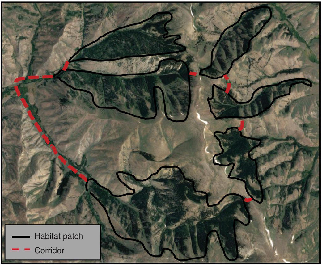
Figure 3.27 Landscape indicating forested habitat patches and connecting corridors in the Lost River Range of central Idaho. Lines show connectivity (linkages) between patches (nodes) of favorable habitat.
Source: Google Images.
We already know that the quantification of a network starts with the measurement of the density of nodes (number of nodes per unit area) and the linear density of the network (total length of lines per unit area) and the pattern of their distribution.
We should now consider another aspect of the network, its connectivity.
3.8 Network Connectivity
Connectivity is measured by the degree to which all nodes in a system are linked by corridors. The quantification of connectivity may use the index (ICON) that relates the observed number of links in the network (ONL) with the maximum number of links (MNL) for a network with the same number of nodes (V) (Figure 3.28). The index25 ICON is therefore calculated as
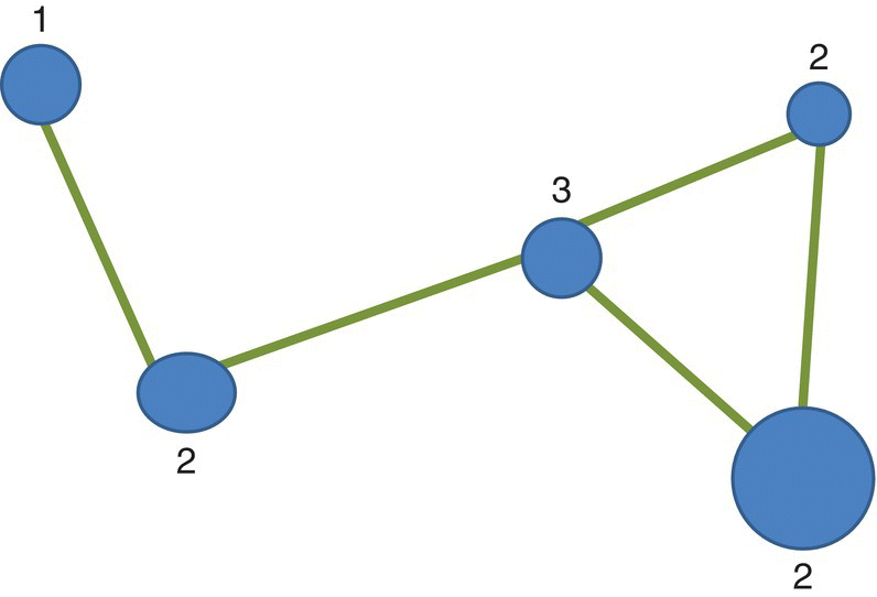
Figure 3.28 Network showing the degree of the different nodes.
The value 3(V – 2) is the maximum number of links in a network assuming that all intersections between links are considered nodes. This index of connectivity ranges from 0 (isolated nodes) to 1 (all nodes connected to all other nodes). The number of linkages of a node (the degree of the node) is also a good indicator of the network pattern.
In this example we have five nodes (V = 5) connected by five links (ONL = 5). The connectivity index is thus
The network is only partially connected. The number of links at each node is in the image and indicates that more linkages could be possible.
Networks may approach three basic forms (topologies): linear (one railroad), dendritic (stream network), and rectilinear (hedgerow) (Figure 3.29).
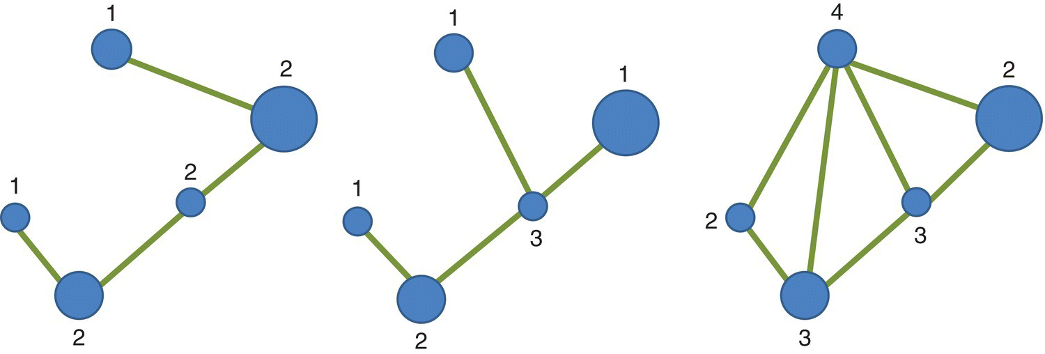
Figure 3.29 Linear, dendritic, and rectilinear networks with 5 nodes (V = 5). In this example, the maximum number of links is MNL = 3(V – 2) = 9. In the first two networks the number of links is 4 (ONL = 4) and therefore we have a connectivity of ICON = 4/9 = 0.44 whereas for the last network we have 7 links and a value of connectivity of ICON = 7/9 = 0.77.
Very simple linear networks generally have 2 linkages originating at each node and vertices have only 1 linkage. For dendritic networks, such as stream systems, nodes with a degree of 1 (vertices) and 3 are common. Rectilinear networks, common for road systems and hedgerows, typically have many nodes originating 3 and 4 linkages.
It is often of interest to maximize network connectivity, as in the case of evaluating alternative greenway networks and linkages26,27. However, the distance between nodes can also be taken into account. In this case the ratio between the number of linkages and their total length can provide a good way to evaluate alternative scenarios or to compare different landscapes. Also, it is possible in transportation theory to derive network topologies to solve basic problems. If we want all nodes to be minimally linked, the solution is a simple linear network, as shown in the example, where nodes are either extreme (degree one) or degree two. For a “traveling salesman” problem of a minimal loop network a solution is obtained for all nodes having a degree of two28.
The use of representation of landscape features as nodes and links may be well demonstrated in the process of designing a network of reserves. In this case nodes represent important habitat patches and links may represent the shortest pathways among those patches. These problems can be solved in the framework of graph theory, as demonstrated in several studies since the pioneer work of Ricotta et al.29
These studies based on graph theory allow for many simulations of the effects of options on the reserve network. One of the common options is the establishment of the minimum spanning tree, which is the shortest path between all nodes that does not include cycles (paths of three or more nodes). These minimum spanning trees can then be assessed as landscape graphs for features as recruitment, dispersal flux, or traversability, and the sensitivity of node removal can be evaluated indicating their relative importance for the network, as shown in Figure 3.30.
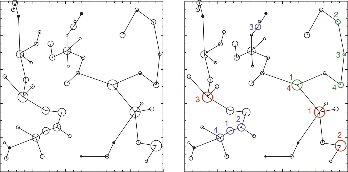
Figure 3.30 Left: hypothetical landscape with 50 circular habitat patches connected by a minimum spanning tree based on dispersal probabilities between patches. Right: results of a node removal exercise showing the most important patches (ranked 1–4) for recruitment (red), dispersal flux (blue), and traversability (green)30.
Other studies follow related approaches31 with the same objective of designing reserve networks based on species characteristics and connectivity.
This is the case of the design of a reserve network in the Vermillion area in the province of Quebec, Canada (Figure 3.31). In this study potential reserve patches were identified as nodes and a minimum planar graph was established with the maximum number of noncrossing links among nodes that are of shortest length. Then the importance of the patches was determined at multiple scales corresponding to the different dispersal abilities of the species to protect. The final reserve network was designed as the overlap of the patches identified as most important for landscape connectivity for each of the species.
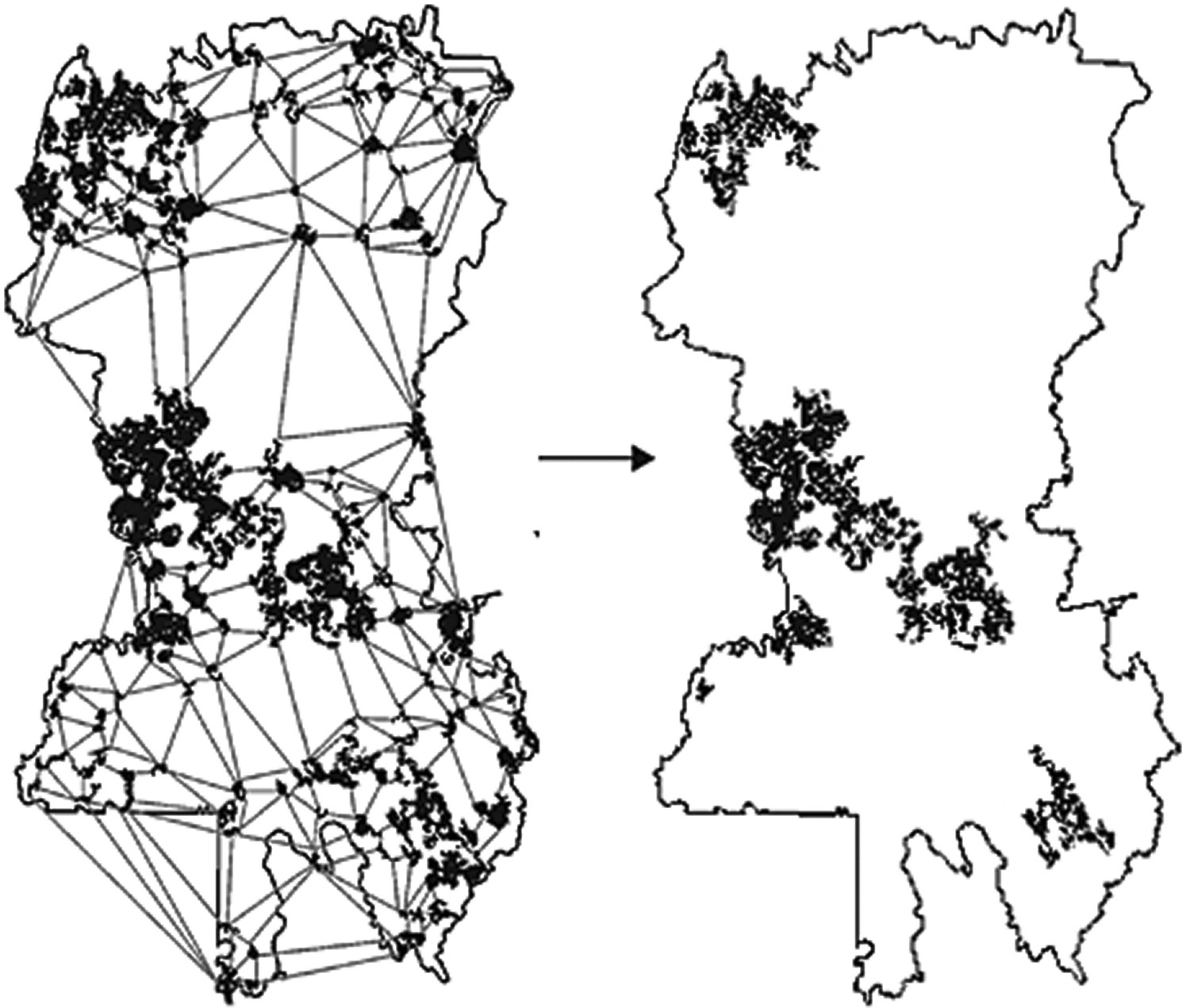
Figure 3.31 Design of a reserve network for the Vermillion area in Quebec, Canada32. The minimum planar graph (left) links all nodes (patches) with the maximum number of links and shortest length. The final reserve network proposed (right) aims at maintaining the maximum landscape connectivity for the species considered (brown creeper (Certhia americana), pileated woodpecker (Dryocopus pileatus), and American marten (Martes americana)).
These two studies illustrate different possibilities of using the approach of graph theory with nodes and links to design reserve networks in the landscape that take into account the ecological characteristics of the species to protect.
3.9 Connectivity Indices Based on Topological Distances Between Patches (Nodes)
Some relatively simple indices based on the topological distance between nodes are available and will be illustrated in this chapter. These indices are based on the work of Frank Harary on graph theory in the United States and have been developed and used in many different situations, such as in evaluating the connectivity in forested or grassland dominated landscapes, by many authors.
In Europe scientists such as Carlo Ricotta and Santiago Saura have been very influential in developing and promoting the use of indices based on graph theory and topological distances between nodes to evaluate connectivity in landscapes (Figure 3.32).

Figure 3.32 Two influential scientists using graph theory in landscape analyses: Frank Harary (1921–2005), American mathematician and one of the “fathers” of graph theory (left), and Carlo Ricotta, Professor of Landscape Ecology at the University of Rome “La Sapienza” (right).
Sources: New Mexico State University (http://newscenter.nmsu.edu/Articles/view/4538) (left), Carlo Riccota (right).
The topological distances between two nodes (dij) is simply the minimum number of links that connect them.
In Figure 3.33 we use the same example as in Figure 3.29 to illustrate the calculations of all the topological distances between all pairs of nodes and the calculation of one of the first indices of connectivity based on topological distances between nodes: the Harary index (HI) computed as the sum of the inverse values of the topological distance (minimum number of links) between every two nodes. If two nodes are not connected, their topological distance is infinity. The index HI can be simply computed by the equation:
where dij is the topological distance (the minimum number of links) between different nodes i and j.
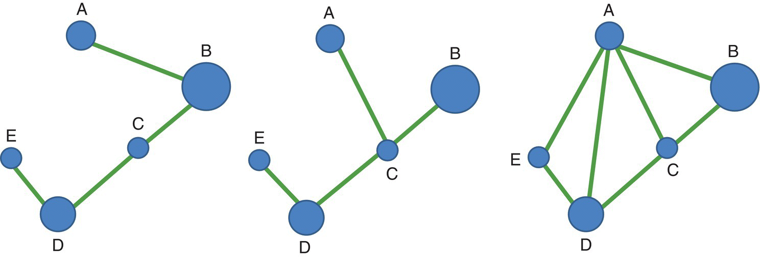
Figure 3.33 The three networks already presented in Figure 3.29 are used in the analysis of connectivity based on topological distances between nodes.
The calculations of the Harary index (HI) for the three networks represented in Figure 3.33 are now presented. The half‐matrices with the topological distances between pairs of nodes are shown for the three networks, followed by the half‐matrices with the inverse of the distances at the bottom, with the corresponding sum, the value of the Harary index (HI):

The first example (left) shows a linear chain network where the nodes are increasingly distant from each other and HI = 6.42 (the minimum value for a linked network of 5 nodes); in the center the value of the connectivity index HI is slightly higher, HI = 6.67, and on the right a very connected network, HI = 8.50.
The Harary index has been used in many studies after it has been presented and described in pioneer works that quantify network connectivity of landscape mosaics based on graph theory33. However, after reviewing many of the existing connectivity indices, Saura and Pascual‐Hortal34,35 identified a number of shortcomings and proposed the integral index of connectivity (IIC). As with the Harary index, the IIC is also calculated from the topological distances between nodes (patches) but it includes attributes of the patches, typically their area, as it influences the estimated dispersal flux between different patches. In this approach the ecological system is modeled as habitat patches (nodes) and connections (links). Any loss or change of either nodes or their links results in a reduction of landscape connectivity for a particular species or process.
Two complementary metrics of landscape connectivity have been used in recent studies.
The first is the number of habitat components. A component is defined as a set of habitat patches with a connection between every two habitat patches within it. As the landscape becomes more connected, the number of components within the landscape decreases36. Also, a threshold distance must be specified for a link to be considered to exist. Obviously, as the threshold distance increases the number of components (nonconnected groups of patches) decreases.
The second connectivity metric is the integral index of connectivity (IIC), based on graph theory, and is capable of combining many spatially explicit habitat variables and species‐specific characteristics into a landscape connectivity value37,38. The equation for the IIC is
where ai and aj are the quantitative characteristic attributes of the node such as area (or habitat quality that may be relevant), dij is the topological distance or the number of links in the shortest path between patches i and j, and MAX is the maximum value of a given landscape attribute, for example the total area of the landscape or the total area of the patch type considered.
Using the networks shown in Figure 3.33 we can illustrate the calculation of IIC. The size of the patches (nodes) was established as
| Patch | Size of patch (hectares) |
| A | 2 |
| B | 5 |
| C | 1 |
| D | 3 |
| E | 1 |
To simplify calculations we consider MAX to be the total area of the patches considered, M = 12 hectares. We can now compute the values for each pair of nodes. For example, for the first network, for the pair of nodes A and B the sizes are 2 and 5 and the topological distance is 1. Therefore the corresponding value is (2 × 5)/(1 + 1) = 5.00. We can now compute all the values for the half matrices (j > i), their sum, and the value of IIC (the sum of the elements of the half‐matrix divided by MAX2) for the three networks:

The results show again that the network at the right is more connected than those at the left and center.
The IIC has been successfully utilized in assessing landscape connectivity in many vegetation types from throughout the world39. Fourie and others used the IIC to assess connectivity in South African landscapes, considering only grassland patches or both grassland and abandoned agricultural lands in the analysis40. Due to the lack of information available on the dispersal distances for many species present, a range of dispersal distances were assessed including: 40, 100, 250, 500, and 1000 m. Obviously, when using larger threshold distances grassland patches were considered to be more connected (low number of components and higher values for the integral index of connectivity). When abandoned agricultural lands were included in the analysis the connectivity of the landscape increased (Figures 3.34 and 3.35).
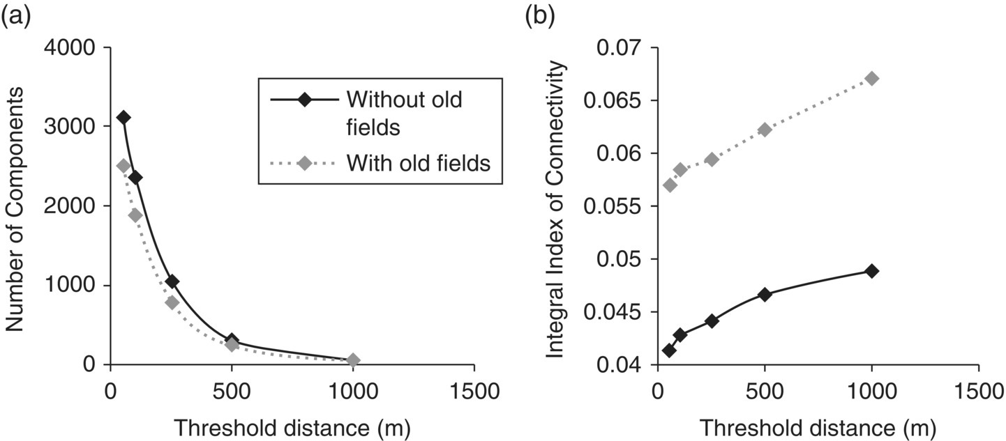
Figure 3.34 (a) Number of components and (b) integral index of connectivity of the grassland habitat patches of Mpumalanga, including and excluding abandoned croplands (old fields).
Source: Fourie, L., Rouget, M., and Lötter, M. (2015) Landscape connectivity of the grassland biome in Mpumalanga, South Africa. Australian Ecology, 40, 67–76.

Figure 3.35 The Blyde River Canyon Nature Reserve, Panorama Route, Mpumalanga, South Africa.
Source: https://commons.wikimedia.org/wiki/File:20131119_162559b.jpg.
The importance of each individual patch for the overall connectivity of the patch type can now be calculated by removing that patch and calculating the new IIC after removal of the patch (IICafter). The percent reduction of the integral index of connectivity for the landscape is the connectivity value of the patch (dIIC):
where IIC is the overall index value when all nodes are present in the landscape and IICafter is the overall index value after the removal of the specific habitat patch41,42.
The results for the grasslands patches of Mpumalanga43 can illustrate the situation (Figure 3.36).

Figure 3.36 The percent differences in the value of the integral index of connectivity (IIC) expressed as percentages dIIC(%) for the grassland patches of Mpumalanga showing that the importance of the individual patches for the connectivity of that habitat in the landscape is geographically highly variable.
Source: Fourie, L., Rouget, M., and Lötter, M. (2015) Landscape connectivity of the grassland biome in Mpumalanga, South Africa. Australian Ecology, 40, 67–76.
The calculation of the values of the integral index of connectivity (IIC) for a certain patch type in the landscape for individual patches of that type (dIIC) can be performed using computer programs that have been incorporated in the system Conefor, making it readily usable by landscape ecologists and planners.44
Although the focus of this chapter is on linear elements and networks more developments on using information on patch attributes as patch size and shape and interactions between patches are presented in the next chapter.
Key Points
- Linear features, which can be line corridors or strip corridors (depending on scale and the objective of the analysis), influence many ecological characteristics and processes in the landscape. Their function can be of conduit, barrier and/or filter, habitat, source and/or sink.
- Linear elements can be represented by single lines, with no width, and are always characterized by length and curvilinearity. The quantification of length depends on the unit of measurement and therefore on the scale of the analysis. The concept of the fractal dimension D is used to measure the curvilinearity of a line and helps to explain how length changes with scale.
- A perfectly straight line has a value D of 1 (D = 1) and the measured length is always independent of the size of the ruler or the scale of the analysis. As the curvilinearity of a line increases, the value D will range between 1 and 2 (1 ≤ D < 2) and the length of the line depends upon the ruler used to measure it and on the scale of the analysis.
- The box‐counting method uses quadrats of different sides to measure the curvilinearity of lines. The length of the line will be the number of quadrats filling the line. As in fractal dimensions, the size of a straight line is independent of the quadrat side and as curvilinearity increases the length of the line depends upon the quadrat side and on the scale of the analysis.
- Linear networks can be described by their density and spatial distribution. They affect ecological processes depending on the type of network and the process considered.
- Density, the most important characteristic of a network of lines, measures the abundance of lines and/or corridors in an area, and is defined as the total length of linear elements per unit area.
- Several methods can be used to determine the spatial pattern or distribution of a network of lines. Methods are based on quadrats, to estimate the fractal dimension of the network of lines, or on distances, to calculate the nearest‐neighbor distance between lines.
- The topology of the networks combines points (nodes) and lines (linkages), and is described by the density of nodes (number of nodes per unit area), by the linear density of the network (total length of lines per unit area), and by the pattern of their distribution.
- Connectivity, another characteristic of networks, is measured by the degree to which all nodes (points) in a system are linked by corridors (lines). Depending on their connectivity, networks may approach three basic forms: linear, dendritic, and/or rectilinear.
- Quantification of connectivity may use simple indices relating the number of nodes and links or indices based on graph theory that use the concept of topological distances between nodes and may include attributes of nodes (as patch sizes).