In Chapter 6, we covered feedforward neural networks, which are the most basic artificial neural network types. Then, we covered convolutional neural networks in Chapter 7 as the type of artificial neural network architecture, which performs exceptionally good on image data. Now, it is time to cover another type of artificial neural network architecture, recurrent neural network, or RNN, designed particularly to deal with sequential data.
Sequence Data and Time-Series Data
RNNs are extremely useful for sequence data. If you are familiar with predictive analytics, you might know that forecasting with time-series data requires different methods compared to cross-sectional data.
Cross-sectional data refers to a set of observations recorded at a single point in time. The percentage returns of a number of different stocks for this year-end would be an example of cross-sectional data.
Time-series data refers to a set of observations recorded over a given period of time at equally spaced time intervals. The percentage returns of a single stock per year in the last 10 years would be an example of time-series data.
In time-series datasets, observations are recorded based on a timestamp, but this cannot be generalized to sequence data. Sequence data refers to a broader term. Sequence data is any data where the order of observations matters. So, time series is a particular type of sequence data ordered by timestamps. For example, the order of a sentence (consisting of several words) is essential for its meaning. We cannot just randomly change the order of words and expect it to mean something. However, words in a sentence are not timestamped, so they do not carry any information on time. Therefore, they are only sequence data, not time-series data. Another example of sequence data (but not time-series data) would be a DNA sequence. The order of a DNA sequence is essential, and they are not ordered based on a timestamp. The relationship between sequence data and time-series data is shown in Figure 8-1.
Figure 8-1
The Relationship Between Sequence Data and Time-Series Data
Now that you know the relationship between time-series data and – the broader term – sequence data, you also know that when we refer to sequence data, we also refer to time-series data, unless stated otherwise.
RNNs usually do a better job in sequence data problems compared to the alternative neural network architectures. Therefore, it is important to know how to implement recurrent neural networks for sequence data problems such as stock price prediction, sales prediction, DNA sequence modeling, and machine translation.
RNNs and Sequential Data
There are three main limitations of feedforward neural networks which makes them unsuitable for sequence data:
A feedforward neural network cannot take the order into account.
A feedforward neural network requires a fixed input size.
A feedforward neural network cannot output predictions in different lengths.
One of the fundamental characteristics of sequence data is the significance of its order. Rearranging the order of monthly sales can lead us from an increasing trend to a decreasing trend, and our prediction for the next month’s sales would change dramatically. This is where the feedforward neural network’s limitation surfaces. In a feedforward neural network, the order of the data cannot be taken into account due to this limitation. Rearranging the order of monthly sales would give the exact same result, which proves that they cannot make use of the order of the inputs.
In sequence data studies, the nature of the problems varies, as shown in Figure 8-2. While a machine translation task is a many-to-many problem in nature, sentiment analysis is a many-to-one task. Especially in tasks where many inputs are possible, we often need a variable input size. However, feedforward neural networks require models to be with fixed input size, which makes them unsuitable for many sequence data problems. If the model is trained to make predictions using the last 7 days, you cannot use the 8th day.
Figure 8-2
Potential Sequence Data Tasks in Deep Learning
Finally, a feedforward neural network cannot output different length predictions. Especially in machine translation problems, we cannot predict the size of the output. For instance, a long sentence in English can easily be expressed with a three-word sentence in a different language. This flexibility cannot be provided with a feedforward neural network. But, RNNs provide this capability, and therefore, they are widely used for tasks like machine translation.
The Basics of RNNs
Let’s take a quick look at the history of RNNs and then briefly cover the real-world use cases of RNNs and their operating mechanism.
The History of RNNs
We already covered some of the RNNs’ history in the previous chapters. The primary motivation to develop RNNs is to eliminate the issues mentioned in the previous section. Over the years, researchers developed different RNN architectures based on their particular research areas. RNNs have many variants, and the total number of different RNN architectures can be expressed in dozens. The first RNN was the Hopfield networks developed by John Hopfield in 1982. In 1997, Hochreiter and Schmidhuber invented long short-term memory (LSTM) networks to address the issues of existing RNNs at the time. LSTM networks perform very well on sequence data tasks, and they are very popular RNN architectures, which are widely used today. In 2014, Kyunghyun Cho introduced recurrent gated units (GRUs) to simplify the LSTM networks. GRUs also perform very well on many tasks, and its inner structure is more straightforward than LSTMs. In this chapter, we will cover simple RNNs, LSTMs, and GRUs in more detail.
Applications of RNNs
There are a significant number of real-world applications of RNNs, and some of these applications can only be built with RNNs. Without RNNs, we would not have competent solutions in many areas, such as machine translation or sentiment analysis. The following is a non-exhaustive list of potential use cases of RNN:
Grammar learning
Handwriting recognition
Human action recognition
Machine translation
Music composition
Predicting subcellular localization of proteins
Prediction in medical care pathways
Protein homology detection
Rhythm learning
Robotics
Sentiment analysis
Speech recognition and synthesis
Time-series anomaly detection
Time-series prediction
Mechanism of RNNs
RNNs make use of previous information by keeping them in memory, which is saved as “state” within an RNN neuron.
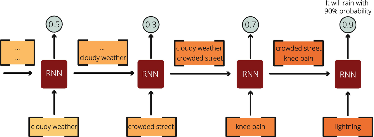
Before diving into the internal structure of LSTMs and GRUs, let’s understand the memory structure with a basic weather forecasting example. We would like to guess if it will rain by using the information provided in a sequence. This sequence of data may be derived from text, speech, or video. After each new information, we slowly update the probability of rainfall and reach a conclusion in the end. Here is the visualization of this task in Figure 8-3.
Figure 8-3
A Simple Weather Forecasting Task: Will It Rain?
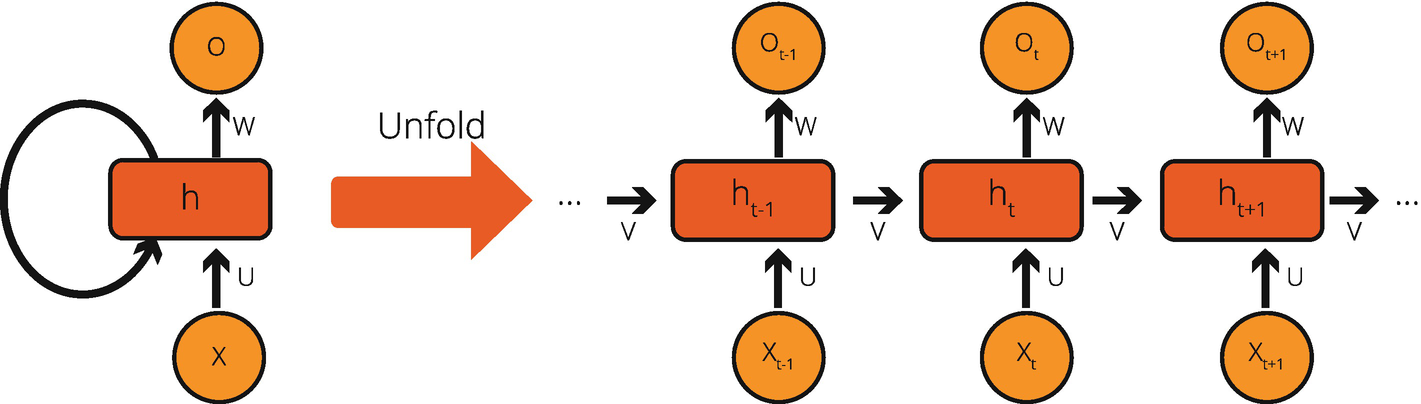
In Figure 8-3, we first record that there is cloudy weather. This single information might be an indication of rain, which calculates into a 50% (or 0.5) probability of rainfall. Then, we receive the following input: crowded street. A crowded street means that people are outside, which means less likelihood of rainfall, and, therefore, our estimation drops to 30% (or 0.3). Then, we are provided with more information: knee pain. It is believed that people with rheumatism feel knee pain before it rains. Therefore, my estimation rises to 70% (or 0.7). Finally, when our model takes lightning as the latest information, the collective estimation increases to 90% (or 0.9). At each time interval, our neuron uses its memory – containing the previous information – and adds the new information on top of this memory to calculate the likelihood of rainfall. The memory structure can be set at the layer level as well as at the cell level. Figure 8-4 shows a cell-level RNN mechanism, (i) folded version on the left and (ii) unfolded version on the right.
Figure 8-4
A Cell-Based Recurrent Neural Network Activity
RNN Types
As mentioned earlier, there are many different variants of RNNs. In this section, we will cover three RNN types we encounter often:
Simple (Simple) RNN
Long short-term memory (LSTM) networks
Gated recurrent unit (GRU) networks
You can find the visualization of these alternative RNN cells in Figure 8-5.
Figure 8-5
Simple RNN, Gated Recurrent Unit, and Long Short-Term Memory Cells
As you can see in Figure 8-5, all these three alternatives have common RNN characteristics:
They all take a t-1 state (memory) into the calculation as a representation of the previous values.
They all apply some sort of activation functions and do matrix operations.
They all calculate a current state at time t.
They repeat this process to perfect their weights and bias values.
Let’s examine these three alternatives in detail.
Simple RNNs
Simple RNNs are a network of neuron nodes, which are designed in connected layers. The inner structure of a simple RNN unit is shown in Figure 8-6.
Figure 8-6
A Simple RNN Unit Structure
In a simple RNN cell, there are two inputs: (i) the state from the previous time step (t-1) and (ii) the observation at the time t. After an activation function (usually Tanh), the output is passed as the state at the time t to the next cell. Therefore, the effect of the previous information is passed to the next cell at each step.
Simple RNNs can solve many sequence data problems, and they are not computationally intensive. Therefore, it might be the best choice in cases where the resources are limited. It is essential to be aware of simple RNNs; however, it is prone to several technical issues such as vanishing gradient problem. Therefore, we tend to use more complex RNN variants such as long short-term memory (LSTM) and gated recurrent unit (GRU).
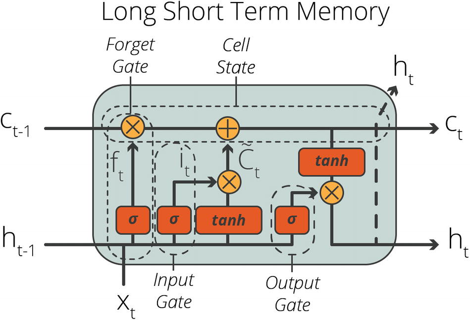
Long Short-Term Memory (LSTM)
Long short-term memory (LSTM) networks are invented by Hochreiter and Schmidhuber in 1997 and improved the highest accuracy performances in many different applications, which are designed to solve sequence data problems.
An LSTM unit consists of a cell state, an input gate, an output gate, and a forget gate, as shown in Figure 8-7. These three gates regulate the flow of information into and out of the LSTM unit. In addition, LSTM units have both a cell state and a hidden state.
Figure 8-7
A Long Short-Term Memory Unit Structure
LSTM networks are well suited for sequence data problems in any format, and they are less prone to vanishing gradient problems, which are common in simple RNN networks. On the other hand, we might still encounter with exploding gradient problem, where the gradients go to the infinity. Another downside of LSTM networks is their computationally intensive nature. Training a model using LSTM might take a lot of time and processing power, which is the main reason why GRUs are developed.
Gated Recurrent Units (GRUs)
Gated recurrent units are introduced in 2014 by Kyunghyun Cho. Just as LSTMs, GRUs are also gating mechanism in RNNs to deal with sequence data. However, to simplify the calculation process, GRUs use two gates: (i) reset gate and (ii) update gate. GRUs also use the same values for hidden state and cell state. Figure 8-8 shows the inner structure of a gated recurrent unit.
Figure 8-8
A Gated Recurrent Unit Structure
GRUs are useful when computational resources are limited. Even though GRUs outperform LSTMs in some applications, LSTMs usually outperform GRUs. A good strategy when dealing with sequence data to train two models with LSTM and GRU and select the best performing one since the performance of these two alternative gating mechanisms can change case by case.
Case Study | Sentiment Analysis with IMDB Reviews
Now that we covered the conceptual part of recurrent neural networks, it is time for a case study. In general, you don’t have to memorize the inner working structure for simple RNNs, LSTMs, and GRUs to build recurrent neural networks. TensorFlow APIs make it very easy to build RNNs that do well on several tasks. In this section, we will conduct a sentiment analysis case study with the IMDB reviews database, which is inspired by TensorFlow’s official tutorial, titled “Text Classification with an RNN”.1
Preparing Our Colab for GPU Accelerated Training
Before diving into exploring our data, there is one crucial environment adjustment: we need to activate GPU training in our Google Colab Notebook. Activating GPU training is a fairly straightforward task, but failure to do it will keep you in CPU training mode forever.
Please go to your Google Colab Notebook, and select the Runtime ➤ “Change runtime type” menu to enable a GPU accelerator, as shown in Figure 8-9.
As mentioned in earlier chapters, using a GPU or TPU – instead of a CPU – for training usually speeds up the training. Now that we enabled GPU use in our model, we can confirm whether a GPU is activated for training with the following code:
IMDB reviews dataset is a large movie review dataset collected and prepared by Andrew L. Maas from the popular movie rating service, IMDB.2 IMDB reviews is used for binary sentiment classification, whether a review is positive or negative. IMDB reviews contains 25,000 movie reviews for training and 25,000 for testing. All these 50,000 reviews are labeled data that may be used for supervised deep learning. Besides, there is an additional 50,000 unlabeled reviews that we will not use in this case study.
Lucky for us, TensorFlow already processed the raw text data and prepared us a bag-of-words format. In addition, we also have access to the raw text. Preparing the bag of words is a natural language processing (NLP) task, which we will cover in the upcoming Chapter 9. Therefore, in this example, we will barely use any NLP technique. Instead, we will use the processed bag-of-words version so that we can easily build our RNN model to predict whether a review is positive or negative.
TensorFlow Imports for Dataset Downloading
We start with two initial imports that are the main TensorFlow import and the TensorFlow datasets import to load the data:
import tensorflow as tf
import tensorflow_datasets as tfds
Loading the Dataset from TensorFlow
TensorFlow offers several popular datasets, which can directly be loaded from the tensorflow_datasets API. The load() function of the tensorflow_datasets API returns two objects: (i) a dictionary containing train, test, and unlabeled sets and (ii) information and other relevant objects regarding the IMDB reviews dataset. We can save them as variables with the following code:
# Dataset is a dictionary containing train, test, and unlabeled datasets
# Info contains relevant information about the dataset
dataset, info = tfds.load('imdb_reviews/subwords8k',
with_info=True,
as_supervised=True)
Understanding the Bag-of-Word Concept: Text Encoding and Decoding
A bag of words is a representation of text that describes the occurrence of words within a document. This representation is created based on a vocabulary of words. In our dataset, reviews are encoded using a vocabulary of 8185 words. We can access the encoder via the “info” object that we created earlier.
# Using info we can load the encoder which converts text to bag of words
# You can also encode a brand new comment with encode function
review = 'Terrible Movie!.'
encoded_review = encoder.encode(review)
print('Encoded review is {}'.format(encoded_review))
output: Encoded review is [3585, 3194, 7785, 7962, 7975]
We can also decode an encoded review as follows:
# You can easily decode an encoded review with decode function
original_review = encoder.decode(encoded_review)
print('The original review is "{}"'.format(original_review))
output: The original review is "Terrible Movie!."
Preparing the Dataset
We already saved our reviews in the “dataset” object, which is a dictionary with three keys: (i) train, (ii) test, and (iii) unlabeled. By using these keys, we will split our train and test sets with the following code:
# We can easily split our dataset dictionary with the relevant keys
We also need to shuffle our dataset to avoid any bias and pad our reviews so that all of them are in the same length. We need to select a large buffer size so that we can have a well-mixed train dataset. In addition, to avoid the excessive computational burden, we will limit our sequence length to 64.
Padding is a useful method to encode sequence data into contiguous batches. To be able to fit all the sequences to a defined length, we must pad or truncate some sequences in our dataset.
Building the Recurrent Neural Network
Now that our train and test datasets are ready to be fed into the model, we can start building our RNN model with LSTM units.
Imports for Model Building
We use Keras Sequential API to build our models. We also need Dense, Embedding, Bidirectional, LSTM, and Dropout layers to build our RNN model. We also need to import Binary Crossentropy as our loss function since we use binary classification to predict whether a comment is negative or positive. Finally, we use Adam optimizer to optimize our weights with backpropagation. These components are imported with the following lines of code:
from tensorflow.keras.models import Sequential
from tensorflow.keras.layers import (Dense,
Embedding,
Bidirectional,
Dropout,
LSTM)
from tensorflow.keras.losses import BinaryCrossentropy
from tensorflow.keras.optimizers import Adam
Create the Model and Fill It with Layers
We use an Encoding layer, two LSTM layers wrapped in Bidirectional layers, two Dense layers, and a Dropout layer. We start with an embedding layer, which converts the sequences of word indices to sequences of vectors. An embedding layer stores one vector per word. Then, we add two LSTM layers wrapped in Bidirectional layers. Bidirectional layers propagate the input back and forth through the LSTM layers and then concatenate the output, which is useful to learn long-range dependencies. Then, we add to one Dense layer with 64 neurons to increase the complexity, a Dropout layer to fight overfitting. Finally, we add a final Dense layer to make a binary prediction. The following lines of code create a Sequential model and add all the mentioned layers:
model = Sequential([
Embedding(encoder.vocab_size, 64),
Bidirectional(LSTM(64, return_sequences=True)),
Bidirectional(LSTM(32)),
Dense(64, activation="relu"),
Dropout(0.5),
Dense(1)
])
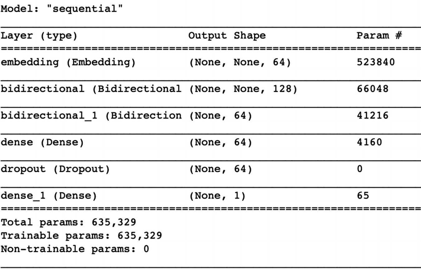
As shown in Figure 8-10, we can also see the overview of the model with model.summary().
Figure 8-10
The Summary of the RNN Model
We can also create a flowchart of our RNN model, as you can see in Figure 8-11, with the following line:
tf.keras.utils.plot_model(model)
Figure 8-11
The Flowchart of the RNN Model
Compiling and Fitting the Model
Now that we build an empty model, it is time to configure the loss function, optimizer, and performance metrics with the following code:
model.compile(
loss=BinaryCrossentropy(from_logits=True),
optimizer=Adam(1e-4),
metrics=['accuracy'])
Our data and model are ready for training. We can use model.fit() function to train our model. Around 10 epochs would be more than enough for training our sentiment analysis model, which may take around 30 minutes. We also save our training process as a variable to access the performance of the model over time.
history = model.fit(train_dataset, epochs=10,
validation_data=test_dataset,
validation_steps=30)
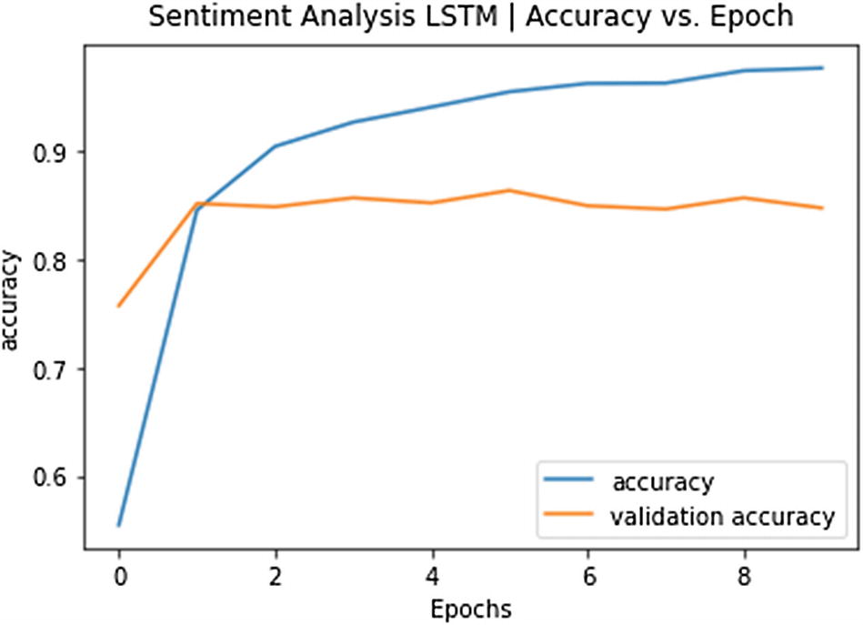
Figure 8-12 shows the main performance measures at each epoch.
Figure 8-12
Model Training Performance at Each Epoch
Evaluating the Model
After seeing an accuracy performance of around 85%, we can safely move on to evaluating our model. We use test_dataset to calculate our final loss and accuracy values:
Accuracy vs. Epoch Plot for Sentiment Analysis LSTM Model
Making New Predictions
Now that we trained our RNN model, we can make new sentiment predictions from the reviews our model has never seen before. Since we encoded and pad our train and test set, we have to process new reviews the same way. Therefore, we need a padder and an encoder. The following code is our custom padding function:
We also need an encoder function that would encode and process our review to feed into our trained model. The following function completes these tasks:
Now we can easily make predictions from previously unseen reviews. For this task, I visited the page IMDB reviews on the movie Fight Club and selected the following comment:
fight_club_review = 'It has some cliched moments, even for its time, but FIGHT CLUB is an awesome film. I have watched it about 100 times in the past 20 years. It never gets old. It is hard to discuss this film without giving things away but suffice it to say, it is a great thriller with some intriguing twists.'
The reviewer gave 8-star and wrote this comment for Fight Club. Therefore, it is clearly a positive comment. Thanks to the custom functions we defined earlier, making a new prediction is very easy, as shown in the following line:
model.predict(review_encoder(fight_club_review))
output: array([[1.5780725]], dtype=float32)
When the output is larger than 0.5, our model classifies the review as positive, whereas negative if below 0.5. Since our output is 1.57, we confirm that our model successfully predicts the sentiment of the review.
Although our model has more than 85% accuracy, one bias I recognized is with regard to the length of the review. When we select a very short review, no matter how positive it is, we always get a negative result. This issue can be addressed with fine-tuning. Even though we will not conduct fine-tuning in this case study, feel free to work on it to improve the model even further.
Saving and Loading the Model
You have successfully trained an RNN model, and you can finish this chapter. But I would like to cover one more topic: saving and loading the trained model. As you experienced, training this model took about 30 minutes, and Google Colab deletes everything you have done after some time of inactivity. So, you have to save your trained model for later use. Besides, you cannot simply save it to a Google Colab directory because it is also deleted after a while. The solution is to save it to your Google Drive. To be able to use our model at any time over the cloud, we should
Give Colab access to save files to our Google Drive
Save the trained model to the designated path
Load the trained model from Google Drive at any time
Make predictions with the SavedModel object
Give Colab Access to Google Drive
To be able to give access to Colab, we need to run the following code inside our Colab Notebook:
from google.colab import drive
drive.mount('/content/gdrive')
Follow the instructions in the output cell to complete this task.
Save Trained Model to Google Drive
Now that we can access our Google Drive files from Colab Notebooks, we can create a new folder called saved_models and save our SavedModel object to this folder with the following lines of code:
# This will create a 'saved_model' folder under the 'content' folder.
!mkdir -p "/content/gdrive/My Drive/saved_model"
# This will save the full model with its variables, weights, and biases.
After this code, we can load our trained model as long as we keep the saved files in our Google Drive. You can also view the folders and files under the sentiment_analysis folder with the following code:
To be able to load the saved_model, we can use the load attribute of the saved_model object. We just need to pass the exact path that our model is located (make sure Colab has access to your Google Drive), and as soon as we run the code, our model is ready for use:
Also, make sure you run the cells where review_padding() and review_encoder() functions (shared earlier) are defined once more if you restart your runtime.
Note that the loaded model object is exactly the same as our previous model, and it has the standard model functions like as fit(), evaluate(), and predict(). To be able to make predictions, we need to use the predict() function of our loaded model object. We also need to pass our processed review as the embedding_input argument. The following line of code completes these tasks:
fight_club_review = 'It has some cliched moments, even for its time, but FIGHT CLUB is an awesome film. I have watched it about 100 times in the past 20 years. It never gets old. It is hard to discuss this film without giving things away but suffice it to say, it is a great thriller with some intriguing twists.'
loaded.predict(review_encoder(rev))
output: array([[1.5780725]], dtype=float32)
As expected, we get the same output. Therefore, we successfully saved our model, load it, and make predictions. Now you can embed this trained model to a web app, REST API, or mobile app to serve to the world!
Conclusion
In this chapter, we covered recurrent neural networks, a type of artificial neural network, which is designed particularly to deal with sequential data. We covered the basics of RNNs and different types of RNNs (basic RNN, LSTM, GRU neurons). Then, we conducted a case study using the IMDB reviews dataset. Our RNN learned to predict whether a review is positive or negative (i.e., sentiment analysis) by using more than 50,000 reviews.
In the next chapter, we will cover natural language processing, a subfield of artificial intelligence, which deals with text data. In addition, we will build another RNN model in the next chapter, but this time, it will generate text data.