Chapter 7

Topic Modeling

Learning Objectives

By the end of this chapter, you'll be able to:

• Perform basic cleaning techniques for textual data
• Evaluate latent Dirichlet allocation models
• Execute non-negative matrix factorization models
• Interpret the results of topic models
• Identify the best topic model for the given scenario

In this chapter, we will see how topic modeling provides insights into the underlying structure of documents.

Introduction

Topic modeling is one facet of natural language processing (NLP), the field of computer science exploring the relationship between computers and human language, which has been increasing in popularity with the increased availability of textual datasets. NLP can deal with language in almost any form, including text, speech, and images. Besides topic modeling, sentiment analysis, object character recognition, and lexical semantics are noteworthy NLP algorithms. Nowadays, the data being collected and needing analysis less frequently comes in standard tabular forms and more frequently coming in less structured forms, including documents, images, and audio files. As such, successful data science practitioners need to be fluent in methodologies used for handling these diverse datasets.

Here is a demonstration of identifying words in a text and assigning them to topics:

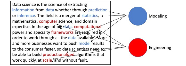
Figure 7.1: Example of identifying words in a text and assigning them to topics

Your immediate question is probably what are topics? Let's answer that question with an example. You could imagine, or perhaps have noticed, that on days when major events take place, such as national elections, natural disasters, or sport championships, the posts on social media websites tend to focus on those events. Posts generally reflect, in some way, the day's events, and they will do so in varying ways. Posts can and will have a number of divergent viewpoints. If we had tweets about the World Cup final, the topics of those tweets could cover divergent viewpoints, ranging from the quality of the refereeing to fan behavior. In the United States, the president delivers an annual speech in mid to late January called the State of the Union. With sufficient numbers of social media posts, we would be able to infer or predict high-level reactions – topics – to the speech from the social media community by grouping posts using the specific keywords contained in them.

Topic Models

Topic models fall into the unsupervised learning bucket because, almost always, the topics being identified are not known in advance. So, no target exists on which we can perform regression or classification modeling. In terms of unsupervised learning, topic models most resemble clustering algorithms, specifically k-means clustering. You'll recall that, in k-means clustering, the number of clusters is established first and then the model assigns each data point to one of the predetermined number of clusters. The same is generally true in topic models. We select the number of topics at the start and then the model isolates the words that form that number of topics. This is a great jumping-off point for a high-level topic modeling overview.

Before that, let's check that the correct environment and libraries are installed and ready for use. The following table lists the required libraries and their main purposes:

Figure 7.2: Table showing different libraries and their use

Exercise 27: Setting Up the Environment

To check whether the environment is ready for topic modeling, we will perform several steps. The first of which involves loading all the libraries that will be needed in this chapter:

Note

If any or all of these libraries are not currently installed, install the required packages via the command line using pip. For example, pip install langdetect, if not installed already.

1. Open a new Jupyter notebook.
2. Import the requisite libraries:

   import langdetect

   import matplotlib.pyplot

   import nltk

   import numpy

   import pandas

   import pyLDAvis

   import pyLDAvis.sklearn

   import regex

   import sklearn

   Note that not all of these packages are used for cleaning the data; some of them are used in the actual modeling, but it is nice to import all of the required libraries at once, so let's take care of all library importing now.

3. Libraries not yet installed will return the following error:
   

   Figure 7.3: Library not installed error

   If this error is returned, install the relevant libraries via the command line as previously discussed. Once successfully installed, rerun the library import process using import.

4. Certain textual data cleaning and preprocessing processes require word dictionaries (more to come). In this step, we will install two of these dictionaries. If the nltk library is imported, the following code can be executed:

   nltk.download('wordnet')

   nltk.download('stopwords')

   The output is as follows:

   

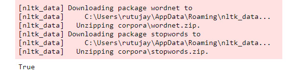
   Figure 7.4: Importing libraries and downloading dictionaries

5. Run the matplotlib magic and specify inline so that the plots print inside the notebook:

   %matplotlib inline

The notebook and environment are now set and ready for data loading.

A High-Level Overview of Topic Models

When it comes to analyzing large volumes of potentially related text data, topic models are one go-to approach. By related, we mean that the documents ideally come from the same source. That is, survey results, tweets, and newspaper articles would not normally be analyzed simultaneously in the same model. It is certainly possible to analyze them together, but the results are liable to be very vague and therefore meaningless. To run any topic model, the only data requirement is the documents themselves. No additional data, meta or otherwise, is required.

In the simplest terms, topic models identify the abstract topics (also known as themes) in a collection of documents, referred to as a corpus, using the words contained in the documents. That is, if a sentence contains the words salary, employee, and meeting, it would be safe to assume that that sentence is about, or that its topic is, work. It is of note that the documents making up the corpus need not be documents as traditionally defined – think letters or contracts. A document could be anything containing text, including tweets, news headlines, or transcribed speech.

Topic models assume that words in the same document are related and use that assumption to define abstract topics by finding groups of words that repeatedly appear in close proximity. In this way, these models are classic pattern recognition algorithms where the patterns being detected are made up of words. The general topic modeling algorithm has four main steps:

1. Determine the number of topics.
2. Scan the documents and identify co-occurring words or phrases.
3. Auto-learn groups (or clusters) of words characterizing the documents.
4. Output abstract topics characterizing the corpus as word groupings.

As step 1 notes, the number of topics needs to be selected before fitting the model. Selecting an appropriate number of topics can be tricky, but, as is the case with most machine learning models, this parameter can be optimized by fitting several models using different numbers of topics and selecting the best model based on some performance metric. We'll dive into this process again later.

The following is the generic topic modeling workflow:

Figure 7.5: The generic topic modeling workflow

It is important to select the best number of topics possible, as this parameter can majorly impact topic coherence. This is because the model finds groups of words that best fit the corpus under the constraint of a predefined number of topics. If the number of topics is too high, the topics become inappropriately narrow. Overly specific topics are referred to as over-cooked. Likewise, if the number of topics is too low, the topics become generic and vague. These types of topics are considered under-cooked. Over-cooked and under-cooked topics can sometimes be fixed by decreasing or increasing the number of topics, respectively. A frequent and unavoidable result of topic models is that, frequently, at least one topic will be problematic.

A key aspect of topic models is that they do not produce specific one-word or one-phrase topics, but rather collections of words, each of which represents an abstract topic. Recall the imaginary sentence about work from before. The topic model built to identify the topics of some hypothetical corpus to which that sentence belongs would not return the word work as a topic. It would instead return a collection of words, such as paycheck, employee, and boss; words that describe the topic and from which the one-word or one-phrase topic could be inferred. This is because topic models understand word proximity, not context. The model has no idea what paycheck, employee, and boss mean; it only knows that these words, generally, whenever they appear, appear in close proximity to one another:

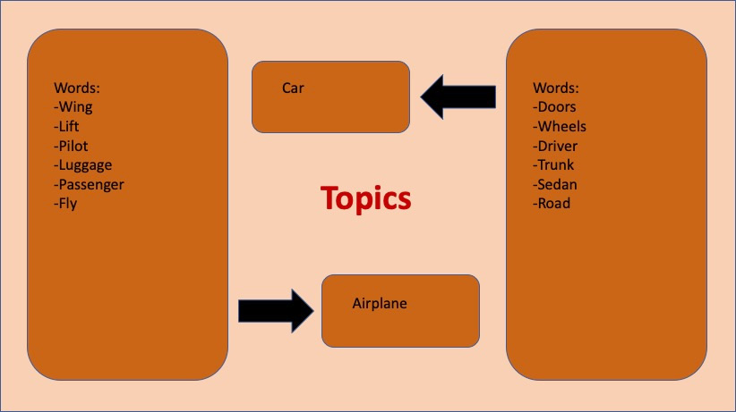
Figure 7.6: Inferring topics from word groupings

Topic models can be used to predict the topic(s) belonging to unseen documents, but, if you are going to make predictions, it is important to recognize that topic models only know the words used to train them. That is, if the unseen documents have words that were not in the training data, the model will not be able to process those words even if they link to one of the topics identified in the training data. Because of this fact, topic models tend to be used more for exploratory analysis and inference more so than for prediction.

Each topic model outputs two matrices. The first matrix contains words against topics. It lists each word related to each topic with some quantification of the relationship. Given the number of words being considered by the model, each topic is only going to be described by a relatively small number of words. Words can either be assigned to one topic or to multiple topics at differing quantifications. Whether words are assigned to one or multiple topics depends on the algorithm. Similarly, the second matrix contains documents against topics. It lists each document related to a topic with some quantification of how related each document is to that topic.

When discussing topic modeling, it is important to continually reinforce the fact that the word groups representing topics are not related conceptually, only by proximity. The frequent proximity of certain words in the documents is enough to define topics because of an assumption stated previously, which is that all words in the same document are related. However, this assumption may either not be true or the words may be too generic to form coherent topics. Interpreting abstract topics involves balancing the innate characteristics of text data with the generated word groupings. Text data, and language in general, is highly variable, complex, and has context, which means any generalized result needs to be consumed cautiously. This is not to downplay or invalidate the results of the model. Given thoroughly cleaned documents and an appropriate number of topics, word groupings, as we will see, can be a good guide as to what is contained in a corpus and can effectively be incorporated into larger data systems.

We have discussed some of the limitations of topic models already, but there are some additional points to consider. The noisy nature of text data can lead topic models to assign words unrelated to one of the topics to that topic. Again, consider the sentence about work from before. The word meeting could appear in the word grouping representing the topic work. It is also possible that the word long could be in that group, but the word long is not directly related to work. Long may be in the group because it frequently appears in close proximity to the word meeting. Therefore, long would probably be considered to be spuriously correlated to work and should probably be removed from the topic grouping, if possible. Spuriously correlated words in word groupings can cause significant problems when analyzing data.

This is not necessarily a flaw in the model, it is, instead, a characteristic of the model that, given noisy data, could extract quirks from the data that might negatively impact the results. Spurious correlations could be the result of how, where, or when the data was collected. If the documents were collected only in some specific geographic region, words associated with that region could be incorrectly, albeit accidentally, linked to one or many of the word groupings output from the model. Note that, with additional words in the word group, we could be attaching more documents to that topic than should be attached. It should be straightforward that, if we shrink the number of words belonging to a topic, then that topic will be assigned to fewer documents. Keep in mind that this is not a bad thing. We want each word grouping to contain only words that make sense so that we assign the appropriate topics to the appropriate documents.

There are many topic modeling algorithms, but perhaps the two best known are Latent Dirichlet Allocation and Non-Negative Matrix Factorization. We will discuss both in detail later on.

Business Applications

Despite its limitations, topic modeling can provide actionable insights that drive business value if used correctly and in the appropriate context. Let's now review one of the biggest applications of topic models.

One of the use cases is exploratory data analysis on new text data where the underlying structure of the dataset is unknown. This is the equivalent to plotting and computing summary statistics for an unseen dataset featuring numeric and categorical variables whose characteristics need to be understood before more sophisticated analyses can be reasonably performed. With the results of topic modeling, the usability of this dataset in future modeling exercises is ascertainable. For example, if the topic model returns clear and distinct topics, then that dataset would be a great candidate for further clustering-type analyses.

Effectively, what determining topics does is to create an additional variable that can be used to sort, categorize, and/or chunk data. If our topic model returns cars, farming, and electronics as abstract topics, we could filter our large text dataset down to just the documents with farming as a topic. Once filtered, we could perform further analyses, including sentiment analysis, another round of topic modeling, or any other analysis we could think up. Beyond defining the topics present in a corpus, topic modeling returns a lot of other information indirectly that could also be used to break a large dataset down and understand its characteristics.

A representation of sorting documents is shown here:

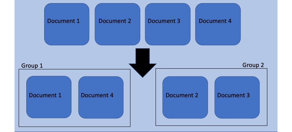
Figure 7.7: Sorting/categorizing documents

Among those characteristics is topic prevalence. Think about performing an analysis on an open response survey that is designed to gauge the response to a product. We could imagine the topic model returning topics in the form of sentiment. One group of words might be good, excellent, recommend, and quality, while the other might be garbage, broken, poor, and disappointing. Given this style of survey, the topics themselves may not be that surprising, but what would be interesting is that we could count the number of documents containing each topic. From the counts, we could say things like x-percent of the survey respondents had a positive reaction to the product, while only y-percent of the respondents had a negative reaction. Essentially, what we would have created is a rough version of a sentiment analysis.

Currently, the most frequent use for a topic model is as a component of a recommendation engine. The emphasis today is on personalization – delivering products to customers that are specifically designed and curated for individual customers. Take websites, news or otherwise, devoted to the propagation of articles. Companies such as Yahoo and Medium need customers to keep reading in order to stay in business, and one way to keep customers reading is to feed them articles that they would be more inclined to read. This is where topic modeling comes in. Using a corpus made up of articles previously read by an individual, a topic model would essentially tell us what types of articles said subscriber likes to read. The company could then go to its inventory and find articles with similar topics and send them to the individual either via their account page or email. This is custom curation to facilitate simplicity and ease of use while also maintaining engagement.

Before we get into prepping data for our model, let's quickly load and explore the data.

Exercise 28: Data Loading

In this exercise we will load the data from a dataset and format it. The dataset for this and all the subsequent exercises in this chapter comes from the Machine Learning Repository, hosted by the University of California, Irvine (UCI). To find the data, go to https://github.com/TrainingByPackt/Applied-Unsupervised-Learning-with-Python/tree/master/Lesson07/Exercise27-Exercise%2038.

Note

This data is downloaded from https://archive.ics.uci.edu/ml/datasets/News+Popularity+in+Multiple+Social+Media+Platforms. It can be accessed at https://github.com/TrainingByPackt/Applied-Unsupervised-Learning-with-Python/tree/master/Lesson07/Exercise27-Exercise%2038. Nuno Moniz and LuÃs Torgo (2018), Multi-Source Social Feedback of Online News Feeds, CoRR UCI Machine Learning Repository [http://archive.ics.uci.edu/ml]. Irvine, CA: University of California, School of Information and Computer Science.

This is the only file that is required for this exercise. Once downloaded and saved locally, the data can be loaded into the notebook:

Note

Execute the exercises of this chapter in the same notebook.

1. Define the path to the data and load it using pandas:

   path = "News_Final.csv"

   df = pandas.read_csv(path, header=0)

   Note

   Add the file on the same path where you have opened your notebook.

2. Examine the data briefly by executing the following code:

   def dataframe_quick_look(df, nrows):

   print("SHAPE: {shape} ".format(shape=df.shape))

   print("COLUMN NAMES: {names} ".format(names=df.columns))

   print("HEAD: {head} ".format(head=df.head(nrows)))

   dataframe_quick_look(df, nrows=2)

   This user-defined function returns the shape of the data (number of rows and columns), the column names, and the first two rows of the data.

   

   Figure 7.8: Raw data

   This is a much larger dataset in terms of features than is needed to run the topic models.

3. Notice that one of the columns, named Topic, actually contains the information that topic models are trying to ascertain. Let's briefly look at the provided topic data, so that when we finally generate our own topics, the results can be compared. Run the following line to print the unique topic values and their number of occurrences:

   print("TOPICS: {topics} ".format(topics=df["Topic"].value_counts()))

   The output is as follows:

   TOPICS:

   economy 33928

   obama 28610

   microsoft 21858

   palestine 8843

   Name: Topic, dtype: int64

4. Now, we extract the headline data and transform the extracted data into a list object. Print the first five elements of the list and the list length to confirm that the extraction was successful:

   raw = df["Headline"].tolist()

   print("HEADLINES: {lines} ".format(lines=raw[:5]))

   print("LENGTH: {length} ".format(length=len(raw)))

Figure 7.9: A list of headlines

With the data now loaded and correctly formatted, let's talk about textual data cleaning and then jump into some actual cleaning and preprocessing. For instructional purposes, the cleaning process will initially be built and executed on only one headline. Once we have established the process and tested it on the example headline, we will go back and run the process on every headline.

Cleaning Text Data

A key component of all successful modeling exercises is a clean dataset that has been appropriately and sufficiently preprocessed for the specific data type and analysis being performed. Text data is no exception, as it is virtually unusable in its raw form. It does not matter what algorithm is being run: if the data isn't properly prepared, the results will be at best meaningless and at worst misleading. As the saying goes, "garbage in, garbage out." For topic modeling, the goal of data cleaning is to isolate the words in each document that could be relevant by removing everything that could be obstructive.

Data cleaning and preprocessing is almost always specific to the dataset, meaning that each dataset will require a unique set of cleaning and preprocessing steps selected to specifically handle the issues in the dataset being worked on. With text data, cleaning and preprocessing steps can include language filtering, removing URLs and screen names, lemmatizing, and stop word removal, among others. In the forthcoming exercises, a dataset featuring news headlines is cleaned for topic modeling.

Data Cleaning Techniques

To reiterate a previous point, the goal of cleaning text for topic modeling is to isolate the words in each document that could be relevant to finding the abstract topics of the corpus. This means removing common words, short words (generally more common), numbers, and punctuation. No hard and fast process exists for cleaning data, so it is important to understand the typical problem points in the type of data being cleaned and to do extensive exploratory work.

Let's now discuss some of the text data cleaning techniques that we will employ. One of the first things that needs to be done when doing any modeling task involving text is to determine the language(s) of the text. In this dataset, most of the headlines are English, so we will remove the non-English headlines for simplicity. Building models on non-English text data requires additional skill sets, the least of which is fluency in the particular language being modeled.

The next crucial step in data cleaning is to remove all elements of the documents that are either not relevant to word-based models or are potential sources of noise that could obscure the results. Elements needing removal could include website addresses, punctuation, numbers, and stop words. Stop words are basically simple, everyday words, including we, are, and the. It is important to note that there is no definitive dictionary of stop words; instead, every dictionary varies slightly. Despite the differences, each dictionary represents a number of common words that are assumed to be topic agnostic. Topic models try to identify words that are both frequent and infrequent enough to be descriptive of an abstract topic.

The removal of website addresses has a similar motivation. Specific website addresses will appear very rarely, but even if one specific website address appears enough to be linked to a topic, website addresses are not interpretable in the same way as words. Removing irrelevant information from the documents reduces the amount of noise that could either prevent model convergence or obscure results.

Lemmatization, like language detection, is an important component of all modeling activities involving text. It is the process of reducing words to their base form as a way to group words that should all be the same but are not. Consider the words running, runs, and ran. All three of these words have the base form of run. A great aspect of lemmatizing is that it looks at all the words in a sentence, or in other words it considers the context, before determining how to alter each word. Lemmatization, like most of the preceding cleaning techniques, simply reduces the amount of noise in the data, so that we can identify clean and interpretable topics.

Now, with basic knowledge of textual cleaning techniques, let's apply it to real-world data.

Exercise 29: Cleaning Data Step by Step

In this exercise, we will learn how to implement some key techniques for cleaning text data. Each technique will be explained as we work through the exercise. After every cleaning step, the example headline is output using print, so we can watch the evolution from raw data to modeling-ready data:

1. Select the fifth headline as the example on which we will build and test the cleaning process. The fifth headline is not a random choice; it was selected because it contains specific problems that will be addressed during the cleaning process:

   example = raw[5]

   print(example)

   The output is as follows:

   

   Figure 7.10: The fifth headline

2. Use the langdetect library to detect the language of each headline. If the language is anything other than English ("en"), remove that headline from the dataset:

   def do_language_identifying(txt):

   try: the_language = langdetect.detect(txt)

   except: the_language = 'none'

   return the_language

   print("DETECTED LANGUAGE: {lang} ".format(lang=do_language_identifying(example)

   ))

   The output is as follows:

   

   Figure 7.11: Detected language

3. Split the string containing the headline into pieces, called tokens, using the white spaces. The returned object is a list of words and numbers that make up the headline. Breaking the headline string into tokens makes the cleaning and preprocessing process simpler:

   example = example.split(" ")

   print(example)

   The output is as follows:

   

   Figure 7.12: String split using white spaces

4. Identify all URLs using a regular expression search for tokens containing http:// or https://. Replace the URLs with the 'URL' string:

   example = ['URL' if bool(regex.search("http[s]?://", i))else i for i in example]

   print(example)

   The output is as follows:

   

   Figure 7.13: URLs replaced with the URL string

5. Replace all punctuation and newline symbols ( ) with empty strings using regular expressions:

   example = [regex.sub("[^\w\s]| ", "", i) for i in example]

   print(example)

   The output is as follows:

   

   Figure 7.14: Punctuation replaced with newline character

6. Replace all numbers with empty strings using regular expressions:

   example = [regex.sub("^[0-9]*$", "", i) for i in example]

   print(example)

   The output is as follows:

   

   Figure 7.15: Numbers replaced with empty strings

7. Change all uppercase letters to lowercase. Converting everything to lowercase is not a mandatory step, but it does help reduce complexity. With everything lowercase, there is less to keep track of and therefore less chance of error:

   example = [i.lower() if i not in "URL" else i for i in example]

   print(example)

   The output is as follows:

   

   Figure 7.16: Uppercase letters converted to lowercase

8. Remove the "URL" string that was added as a placeholder in step 4. The previously added "URL" string is not actually needed for modeling. If it seems harmless to leave it in, consider that the "URL" string could appear naturally in a headline and we do not want to artificially boost its number of appearances. Also, the "URL" string does not appear in every headline, so by leaving it in we could be unintentionally creating a connection between the "URL" strings and a topic:

   example = [i for i in example if i not in "URL"]

   print(example)

   The output is as follows:

   

   Figure 7.17: String URL removed

9. Load in the stopwords dictionary from nltk and print it:

   list_stop_words = nltk.corpus.stopwords.words("English")

   list_stop_words = [regex.sub("[^\w\s]", "", i) for i in list_stop_words]

   print(list_stop_words)

   The output is as follows:

   

   Figure 7.18: List of stop words

   Before using the dictionary, it is important to reformat the words to match the formatting of our headlines. That involves confirming that everything is lowercase and without punctuation.

10. Now that we have correctly formatted the stopwords dictionary, use it to remove all stop words from the headline:

    example = [i for i in example if i not in list_stop_words]

    print(example)

    The output is as follows:

    

    Figure 7.19: Stop words removed from the headline

11. Perform lemmatization by defining a function that can be applied to each headline individually. Lemmatizing requires loading the wordnet dictionary:

    def do_lemmatizing(wrd):

    out = nltk.corpus.wordnet.morphy(wrd)

    return (wrd if out is None else out)

    example = [do_lemmatizing(i) for i in example]

    print(example)

    The output is as follows:

    

    Figure 7.20: Output after performing lemmatization

12. Remove all words with a length of four of less from the list of tokens. The assumption around this step is that short words are, in general, more common and therefore will not drive the types of insights we are looking to extract from the topic models. This is the final step of data cleaning and preprocessing:

    example = [i for i in example if len(i) >= 5]

    print(example)

    The output is as follows:

Figure 7.21: Headline number five post-cleaning

Now that we have worked through the cleaning and preprocessing steps individually on one headline, we need to apply those steps to every one of the nearly 100,000 headlines. Applying the steps to every headline the way we applied them to the single headline, which is in a manual way, is not feasible.

Exercise 30: Complete Data Cleaning

In this exercise, we will consolidate steps 2 through 12 from Exercise 29, Cleaning Data Step-by-Step, into one function that we can apply to every headline. The function will take one headline in string format as an input and output one cleaned headline as a list of tokens. The topic models require that documents be formatted as strings instead of as lists of tokens, so, in step 4, the lists of tokens are converted back into strings:

1. Define a function that contains all the individual steps of the cleaning process from Exercise 29, Cleaning Data Step-by-step:

   def do_headline_cleaning(txt):

   # identify language of tweet

   # return null if language not English

   lg = do_language_identifying(txt)

   if lg != 'en':

   return None

   # split the string on whitespace

   out = txt.split(" ")

   # identify urls

   # replace with URL

   out = ['URL' if bool(regex.search("http[s]?://", i)) else i for i in out]

   # remove all punctuation

   out = [regex.sub("[^\w\s]| ", "", i) for i in out]

   # remove all numerics

   out = [regex.sub("^[0-9]*$", "", i) for i in out]

   # make all non-keywords lowercase

   out = [i.lower() if i not in "URL" else i for i in out]

   # remove URL

   out = [i for i in out if i not in "URL"]

   # remove stopwords

   list_stop_words = nltk.corpus.stopwords.words("English")

   list_stop_words = [regex.sub("[^\w\s]", "", i) for i in list_stop_words]

   out = [i for i in out if i not in list_stop_words]

   # lemmatizing

   out = [do_lemmatizing(i) for i in out]

   # keep words 5 or more characters long

   out = [i for i in out if len(i) >= 5]

   return out

2. Execute the function on each headline. The map function in Python is a nice way to apply a user-defined function to each element of a list. Convert the map object to a list and assign it to the clean variable. The clean variable is a list of lists:

   clean = list(map(do_headline_cleaning, raw))

3. In do_headline_cleaning, None is returned if the language of the headline is detected as being any language other than English. The elements of the final cleaned list should only be lists, not None, so remove all None types. Use print to display the first five cleaned headlines and the length of the clean variable:

   clean = list(filter(None.__ne__, clean))

   print("HEADLINES: {lines} ".format(lines=clean[:5]))

   print("LENGTH: {length} ".format(length=len(clean)))

   The output is as follows:

   

   Figure 7.22: Headline and its length

4. For every individual headline, concatenate the tokens using a white space separator. The headlines should now be an unstructured collection of words, nonsensical to the human reader, but ideal for topic modeling:

   clean_sentences = [" ".join(i) for i in clean]

   print(clean_sentences[0:10])

   The cleaned headlines should resemble the following:

Figure 7.23: Headlines cleaned for modeling

To recap, what the cleaning and preprocessing work effectively does is strip out the noise from the data, so that the model can hone in on elements of the data that could actually drive insights. For example, words that are agnostic to any topic (or stop words) should not be informing topics, but, by accident alone if left in, could be informing topics. In an effort to avoid what we could call "fake signals," we remove those words. Likewise, since topic models cannot discern context, punctuation is irrelevant and is therefore removed. Even if the model could find the topics without removing the noise from the data, the uncleaned data could have thousands to millions of extra words and random characters to parse, depending on the number of documents in the corpus, which could significantly increase the computational demands. So, data cleaning is an integral part of topic modeling.

Activity 15: Loading and Cleaning Twitter Data

In this activity, we will load and clean Twitter data for modeling done in subsequent activities. Our usage of the headline data is ongoing, so let's complete this activity in a separate Jupyter notebook, but with all the same requirements and imported libraries.

The goal is to take the raw tweet data, clean it, and produce the same output that we did in Step 4 of the previous exercise. That output should be a list whose length is similar to the number of rows in the raw data file. The length is similar to, meaning potentially not equal to, the number of rows, because tweets can get dropped in the cleaning process for reasons including that the tweet might not be in English. Each element of the list should represent one tweet and should contain just the words in the tweet that might be relevant to topic formation.

Here are the steps to complete the activity:

1. Import the necessary libraries.
2. Load the LA Times health Twitter data (latimeshealth.txt) from https://github.com/TrainingByPackt/Applied-Unsupervised-Learning-with-Python/tree/master/Lesson07/Activity15-Activity17.

   Note

   This dataset is downloaded from https://archive.ics.uci.edu/ml/datasets/Health+News+in+Twitter. We have uploaded it on GitHub and it can be downloaded from https://github.com/TrainingByPackt/Applied-Unsupervised-Learning-with-Python/tree/master/Lesson07/Activity15-Activity17. Karami, A., Gangopadhyay, A., Zhou, B., & Kharrazi, H. (2017). Fuzzy approach topic discovery in health and medical corpora. International Journal of Fuzzy Systems. UCI Machine Learning Repository [http://archive.ics.uci.edu/ml]. Irvine, CA: University of California, School of Information and Computer Science.

3. Run a quick exploratory analysis to ascertain data size and structure.
4. Extract the tweet text and convert it to a list object.
5. Write a function to perform language detection, tokenization on whitespaces, and replace screen names and URLs with SCREENNAME and URL, respectively. The function should also remove punctuation, numbers, and the SCREENNAME and URL replacements. Convert everything to lowercase, except SCREENNAME and URL. It should remove all stop words, perform lemmatization, and keep words with five or more letters.
6. Apply the function defined in step 5 to every tweet.
7. Remove elements of the output list equal to None.
8. Turn the elements of each tweet back into a string. Concatenate using white space.
9. Keep the notebook open for future modeling.

   Note

   All the activities in this chapter need to be performed in the same notebook.

10. The output will be as follows:

Figure 7.24: Tweets cleaned for modeling

Note

The solution for this activity can be found on page 357.

Latent Dirichlet Allocation

In 2003, David Biel, Andrew Ng, and Michael Jordan published their article on the topic modeling algorithm known as Latent Dirichlet Allocation (LDA). LDA is a generative probabilistic model. This means that we assume the process, which is articulated in terms of probabilities, by which the data was generated is known and then work backward from the data to the parameters that generated it. In this case, it is the topics that generated the data that are of interest. The process discussed here is the most basic form of LDA, but for learning, it is also the most comprehensible.

For each document in the corpus, the assumed generative process is:

1. Select 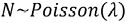, where is the number of words.
2. Select , where is the distribution of topics.
3. For each of the words , select topic , and select word from .

Let's go through the generative process in a bit more detail. The preceding three steps repeat for every document in the corpus. The initial step is to choose the number of words in the document by sampling from, in most cases, the Poisson distribution. It is important to note that, because N is independent of the other variables, the randomness associated with its generation is mostly ignored in the derivation of the algorithm. Coming after the selection of N is the generation of the topic mixture or distribution of topics, which is unique to each document. Think of this as a per-document list of topics with probabilities representing the amount of the document represented by each topic. Consider three topics: A, B, and C. An example document could be 100% topic A, 75% topic B, and 25% topic C, or an infinite number of other combinations. Lastly, the specific words in the document are selected via a probability statement conditioned on the selected topic and the distribution of words for that topic. Note that documents are not really generated in this way, but it is a reasonable proxy.

This process can be thought of as a distribution over distributions. A document is selected from the collection (distribution) of documents, and from that document one topic is selected, via the multinomial distribution, from the probability distribution of topics for that document generated by the Dirichlet distribution:

Figure 7.25: Graphical representation of LDA

The most straightforward way to build the formula representing the LDA solution is through a graphical representation. This particular representation is referred to as a plate notation graphical model, as it uses plates to represent the two iterative steps in the process. You will recall that the generative process was executed for every document in the corpus, so the outermost plate, labeled M, represents iterating over each document. Similarly, the iteration over words in step 3 is represented by the innermost plate of the diagram, labeled N. The circles represent the parameters, distributions, and results. The shaded circle, labeled w, is the selected word, which is the only known piece of data and, as such, is used to reverse-engineer the generative process. Besides w, the other four variables in the diagram are defined as follows:

• : Hyperparameter for the topic-document Dirichlet distribution
• : Distribution of words for each topic
• : This is the latent variable for the topic
• : This is the latent variable for the distribution of topics for each document

and control the frequency of topics in documents and of words in topics. If increases, the documents become increasingly similar as the number of topics in each document increases. On the other hand, if decreases, the documents become increasingly dissimilar as the number of topics in each document decreases. The parameter behaves similarly.

Variational Inference

The big issue with LDA is that the evaluation of the conditional probabilities, the distributions, is unmanageable, so instead of computing them directly, the probabilities are approximated. Variational inference is one of the simpler approximation algorithms, but it has an extensive derivation that requires significant knowledge of probability. In order to spend more time on the application of LDA, this section will give some high-level details on how variational inference is applied in this context, but will not fully explore the algorithm.

Let's take a moment to work through the variational inference algorithm intuitively. Start by randomly assigning each word in each document in the corpus to one of the topics. Then, for each document and each word in each document separately, calculate two proportions. Those proportions would be the proportion of words in the document that are currently assigned to the topic, , and the proportion of assignments across all documents of a specific word to the topic, . Multiply the two proportions and use the resulting proportion to assign the word to a new topic. Repeat this process until a steady state, where topic assignments are not changing significantly, is reached. These assignments are then used to estimate the within-document topic mixture and the within-topic word mixture.

Figure 7.26: The variational inference process

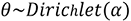
The thought process behind variational inference is that, if the actual distribution is intractable, then a simpler distribution, let's call it the variational distribution, very close to initial distribution, which is tractable, should be found so that inference becomes possible.

To start, select a family of distributions, q, conditioned on new variational parameters. The parameters are optimized so that the original distribution, which is actually the posterior distribution for those people familiar with Bayesian statistics, and the variational distribution are as close as possible. The variational distribution will be close enough to the original posterior distribution to be used as a proxy, making any inference done on it applicable to the original posterior distribution. The generic formula for the family of distributions, q, is as follows:

Figure 7.27: Formula for the family of distributions, q

There is a large collection of potential variational distributions that can be used as an approximation for the posterior distribution. An initial variational distribution is selected from the collection, which acts as the starting point for an optimization process that iteratively moves closer and closer to the optimal distribution. The optimal parameters are the parameters of the distribution that best approximate the posterior.

The similarity of the two distributions is measured using the Kullback-Leibler (KL) divergence. KL divergence is also known as relative entropy. Again, finding the best variational distribution, q, for the original posterior distribution, p, requires minimizing the KL divergence. The default method for finding the parameters that minimize the divergence is the iterative fixed-point method, which we will not dig into here.

Once the optimal distribution has been identified, which means the optimal parameters have been identified, it can be leveraged to produce the output matrices and do any required inference.

Bag of Words

Text cannot be passed directly into any machine learning algorithm; it first needs to be encoded numerically. A straightforward way of working with text in machine learning is via a bag-of-words model, which removes all information around the order of the words and focuses strictly on the degree of presence, meaning count or frequency, of each word. The Python sklearn library can be leveraged to transform the cleaned vector created in the previous exercise into the structure that the LDA model requires. Since LDA is a probabilistic model, we do not want to do any scaling or weighting of the word occurrences; instead, we opt to input just the raw counts.

The input of the bag-of-words model will be the list of cleaned strings that were returned from Exercise 4, Complete Data Cleaning. The output will be the document number, the word as its numeric encoding, and the count of times that word appears in that document. These three items will be presented as a tuple and an integer. The tuple will be something like (0, 325), where 0 is the document number and 325 is the numerically encoded word. Note that 325 would be the encoding of that word across all documents. The integer would then be the count. The bag-of-words models we will be running in this chapter are from sklearn and are called CountVectorizer and TfIdfVectorizer. The first model returns the raw counts and the second returns a scaled value, which we will discuss a bit later.

A critical note is that the results of both topic models being covered in this chapter can vary from run to run, even when the data is the same, because of randomness. Neither the probabilities in LDA nor the optimization algorithms are deterministic, so do not be surprised if your results differ slightly from the results shown from here on out.

Exercise 31: Creating a Bag-of-Words Model Using the Count Vectorizer

In this exercise, we will run the CountVectorizer in sklearn to convert our previously created cleaned vector of headlines into a bag-of-words data structure. In addition, we will define some variables that will be used through the modeling process.

1. Define number_words, number_docs, and number_features. The first two variables control the visualization of the LDA results. More to come later. The number_features variable controls the number of words that will be kept in the feature space:

   number_words = 10

   number_docs = 10

   number_features = 1000

2. Run the count vectorizer and print the output. There are three crucial inputs, which are max_df, min_df, and max_features. These parameters further filter the number of words in the corpus down to those that will most likely influence the model. Words that only appear in a small number of documents are too rare to be attributed to any topic, so min_df is used to throw away words that appear in less than the specified number of documents. Words that appear in too many documents are not specific enough to be linked to specific topics, so max_df is used to throw away words that appear in more than the specified percentage of documents. Lastly, we do not want to overfit the model, so the number of words used to fit the model is limited to the most frequently occurring specified number (max_features) of words:

   vectorizer1 = sklearn.feature_extraction.text.CountVectorizer(

   analyzer="word",

   max_df=0.5,

   min_df=20,

   max_features=number_features

   )

   clean_vec1 = vectorizer1.fit_transform(clean_sentences)

   print(clean_vec1[0])

   The output is as follows:

   

   Figure 7.28: The bag-of-words data structure

3. Extract the feature names and the words from the vectorizer. The model is only fed the numerical encodings of the words, so having the feature names vector to merge with the results will make interpretation easier:

   feature_names_vec1 = vectorizer1.get_feature_names()

Perplexity

Models generally have metrics that can be leveraged to evaluate their performance. Topic models are no different, although performance in this case has a slightly different definition. In regression and classification, predicted values can be compared to actual values from which clear measures of performance can be calculated. With topic models, prediction is less reliable, because the model only knows the words it was trained on and new documents may not contain any of those words, despite featuring the same topics. Due to that difference, topic models are evaluated using a metric specific to language models called perplexity. Perplexity, abbreviated to PP, measures the number of different equally most probable words that can follow any given word on average. Let's consider two words as an example: the and announce. The word the can preface an enormous number of equally most probable words, while the number of equally most probable words that can follow the word announce is significantly less – albeit still a large number.

The idea is that words that, on average, can be followed by a smaller number of equally most probable words are more specific and can be more tightly tied to topics. As such, lower perplexity scores imply better language models. Perplexity is very similar to entropy, but perplexity is typically used because it is easier to interpret. As we will see momentarily, it can be used to select the optimal number of topics. With m being the number of words in the sequence of words, perplexity is defined as:

Figure 7.29: Formula of perplexity

Exercise 32: Selecting the Number of Topics

As stated previously, LDA has two required inputs. The first are the documents themselves and the second is the number of topics. Selecting an appropriate number of topics can be very tricky. One approach to finding the optimal number of topics is to search over several numbers of topics and select the number of topics that corresponds to the smallest perplexity score. In machine learning, this approach is referred to as grid search.

In this exercise, we use the perplexity scores for LDA models fit on varying numbers of topics to determine the number of topics with which to move forward. Keep in mind that the original dataset had the headlines sorted into four topics. Let's see whether this approach returns four topics:

1. Define a function that fits an LDA model on various numbers of topics and computes the perplexity score. Return two items: a data frame that has the number of topics with its perplexity score and the number of topics with the minimum perplexity score as an integer:

   def perplexity_by_ntopic(data, ntopics):

   output_dict = {

   "Number Of Topics": [],

   "Perplexity Score": []

   }

   for t in ntopics:

   lda = sklearn.decomposition.LatentDirichletAllocation(

   n_components=t,

   learning_method="online",

   random_state=0

   )

   lda.fit(data)

   output_dict["Number Of Topics"].append(t)

   output_dict["Perplexity Score"].append(lda.perplexity(data))

   output_df = pandas.DataFrame(output_dict)

   index_min_perplexity = output_df["Perplexity Score"].idxmin()

   output_num_topics = output_df.loc[

   index_min_perplexity, # index

   "Number Of Topics" # column

   ]

   return (output_df, output_num_topics)

2. Execute the function defined in step 1. The ntopics input is a list of numbers of topics that can be of any length and contain any values. Print out the data frame:

   df_perplexity, optimal_num_topics = perplexity_by_ntopic(

   clean_vec1,

   ntopics=[1, 2, 3, 4, 6, 8, 10]

   )

   print(df_perplexity)

   The output is as follows:

   

   Figure 7.30: Data frame containing number of topics and perplexity score

3. Plot the perplexity scores as a function of the number of topics. This is just another way to view the results contained in the data frame from step 2:

   df_perplexity.plot.line("Number Of Topics", "Perplexity Score")

   The plot looks as follows:

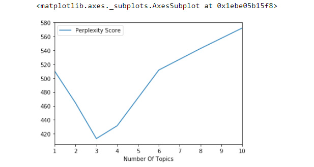
Figure 7.31: Line plot view of perplexity as a function of the number of topics

As the data frame and plot show, the optimal number of topics using perplexity is three. Having the number of topics set to four yielded the second-lowest perplexity, so, while the results did not exactly match with the information contained in the original dataset, the results are close enough to engender confidence in the grid search approach to identifying the optimal number of topics. There could be several reasons that the grid search returned three instead of four, which we will dig into in future exercises.

Exercise 33: Running Latent Dirichlet Allocation

In this exercise, we implement LDA and examine the results. LDA outputs two matrices. The first is the topic-document matrix and the second is the word-topic matrix. We will look at these matrices as returned from the model and as nicely formatted tables that are easier to digest:

1. Fit an LDA model using the optimal number of topics found in Exercise 32, Selecting the Number of Topics:

   lda = sklearn.decomposition.LatentDirichletAllocation(

   n_components=optimal_num_topics,

   learning_method="online",

   random_state=0

   )

   lda.fit(clean_vec1)

   The output is as follows:

   

   Figure 7.32: LDA model

2. Output the topic-document matrix and its shape to confirm that it aligns with the number of topics and the number of documents. Each row of the matrix is the per-document distribution of topics:

   lda_transform = lda.transform(clean_vec1)

   print(lda_transform.shape)

   print(lda_transform)

   The output is as follows:

   

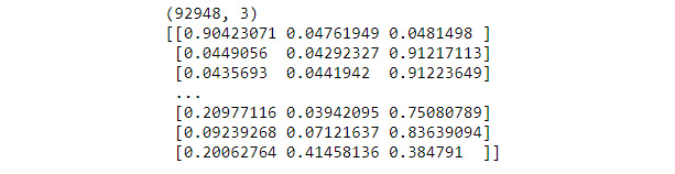
   Figure 7.33: Topic-document matrix and its dimensions

3. Output the word-topic matrix and its shape to confirm that it aligns with the number of features (words) specified in Exercise 31, Creating Bag-of-Words Model Using the Count Vectorizer, and the number of topics input. Each row is basically the counts (although not counts exactly) of assignments to that topic of each word, but those quasi-counts can be transformed into the per-topic distribution of words:

   lda_components = lda.components_

   print(lda_components.shape)

   print(lda_components)

   The output is as follows:

   

   Figure 7.34: Word-topic matrix and its dimensions

4. Define a function that formats the two output matrices into easy-to-read tables:

   def get_topics(mod, vec, names, docs, ndocs, nwords):

   # word to topic matrix

   W = mod.components_

   W_norm = W / W.sum(axis=1)[:, numpy.newaxis]

   # topic to document matrix

   H = mod.transform(vec)

   W_dict = {}

   H_dict = {}

   for tpc_idx, tpc_val in enumerate(W_norm):

   topic = "Topic{}".format(tpc_idx)

   # formatting w

   W_indices = tpc_val.argsort()[::-1][:nwords]

   W_names_values = [

   (round(tpc_val[j], 4), names[j])

   for j in W_indices

   ]

   W_dict[topic] = W_names_values

   # formatting h

   H_indices = H[:, tpc_idx].argsort()[::-1][:ndocs]

   H_names_values = [

   (round(H[:, tpc_idx][j], 4), docs[j])

   for j in H_indices

   ]

   H_dict[topic] = H_names_values

   W_df = pandas.DataFrame(

   W_dict,

   index=["Word" + str(i) for i in range(nwords)]

   )

   H_df = pandas.DataFrame(

   H_dict,

   index=["Doc" + str(i) for i in range(ndocs)]

   )

   return (W_df, H_df)

   The function may be tricky to navigate, so let's walk through it. Start by creating the W and H matrices, which includes converting the assignment counts of W into the per-topic distribution of words. Then, iterate over the topics. Inside each iteration, identify the top words and documents associated with each topic. Convert the results into two data frames.

5. Execute the function defined in step 4:

   W_df, H_df = get_topics(

   mod=lda,

   vec=clean_vec1,

   names=feature_names_vec1,

   docs=raw,

   ndocs=number_docs,

   nwords=number_words

   )

6. Print out the word-topic data frame. It shows the top-10 words, by distribution value, that are associated with each topic. From this data frame, we can identify the abstract topics that the word groupings represent. More on abstract topics to come:

   print(W_df)

   The output is as follows:

   

   Figure 7.35: Word-topic table

7. Print out the topic-document data frame. It shows the 10 documents to which each topic is most closely related. The values are from the per-document distribution of topics:

   print(H_df)

   The output is as follows:

Figure 7.36: Topic-document table

The results of the word-topic data frame show that the abstract topics are Barack Obama, the economy, and Microsoft. What is interesting is that the word grouping describing the economy contains references to Palestine. All four topics specified in the original dataset are represented in the word-topic data frame output, but not in the fully distinct manner expected. We could be facing one of two problems. First, the topic referencing both the economy and Palestine could be under-cooked, which means increasing the number of topics may fix the issue. The other potential problem is that LDA does not handle correlated topics well. In Exercise 35, Trying Four Topics, we will try expanding the number of topics, which will give us a better idea of why one of the word groupings is seemingly a mixture of topics.

Exercise 34: Visualize LDA

Visualization is a helpful tool for exploring the results of topic models. In this exercise, we will look at three different visualizations. Those visualizations are basic histograms and specialty visualizations using t-SNE and PCA.

To create some of the visualizations, we are going to use the pyLDAvis Library. This library is flexible enough to take in topic models built using several different frameworks. In this case, we will use the sklearn framework. This visualization tool returns a histogram showing the words that are the most closely related to each topic and a biplot, frequently used in PCA, where each circle corresponds to a topic. From the biplot, we know how prevalent each topic is across the whole corpus, which is reflected by the area of the circle, and the similarity of the topics, which is reflected by the closeness of the circles. The ideal scenario is to have the circles spread throughout the plot and be of reasonable size. That is, we want the topics to be distinct and to appear consistently across the corpus:

1. Run and display pyLDAvis. This plot is interactive. Clicking on each circle updates the histogram to show the top words related to that specific topic. The following is one view of this interactive plot:

   lda_plot = pyLDAvis.sklearn.prepare(lda, clean_vec1, vectorizer1, R=10)

   pyLDAvis.display(lda_plot)

   The plot looks as follows:

   

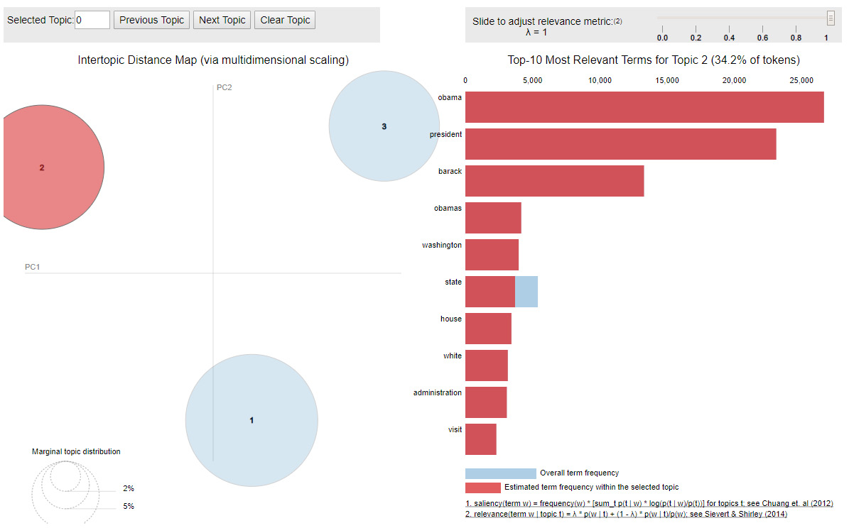
   Figure 7.37: A histogram and biplot for the LDA model

2. Define a function that fits a t-SNE model and then plots the results:

   def plot_tsne(data, threshold):

   # filter data according to threshold

   index_meet_threshold = numpy.amax(data, axis=1) >= threshold

   lda_transform_filt = data[index_meet_threshold]

   # fit tsne model

   # x-d -> 2-d, x = number of topics

   tsne = sklearn.manifold.TSNE(

   n_components=2,

   verbose=0,

   random_state=0,

   angle=0.5,

   init='pca'

   )

   tsne_fit = tsne.fit_transform(lda_transform_filt)

   # most probable topic for each headline

   most_prob_topic = []

   for i in range(tsne_fit.shape[0]):

   most_prob_topic.append(lda_transform_filt[i].argmax())

   print("LENGTH: {} ".format(len(most_prob_topic)))

   unique, counts = numpy.unique(

   numpy.array(most_prob_topic),

   return_counts=True

   )

   print("COUNTS: {} ".format(numpy.asarray((unique, counts)).T))

   # make plot

   color_list = ['b', 'g', 'r', 'c', 'm', 'y', 'k']

   for i in list(set(most_prob_topic)):

   indices = [idx for idx, val in enumerate(most_prob_topic) if val == i]

   matplotlib.pyplot.scatter(

   x=tsne_fit[indices, 0],

   y=tsne_fit[indices, 1],

   s=0.5,

   c=color_list[i],

   label='Topic' + str(i),

   alpha=0.25

   )

   matplotlib.pyplot.xlabel('x-tsne')

   matplotlib.pyplot.ylabel('y-tsne')

   matplotlib.pyplot.legend(markerscale=10)

   The function starts by filtering down the topic-document matrix using an input threshold value. There are tens of thousands of headlines and any plot incorporating all the headlines is going to be difficult to read and therefore not helpful. So, this function only plots a document if one of the distribution values is greater than or equal to the input threshold value. Once the data is filtered down, we run t-SNE, where the number of components is two, so we can plot the results in two dimensions. Then, create a vector with an indicator of which topic is most related to each document. This vector will be used to color-code the plot by topic. To understand the distribution of topics across the corpus and the impact of threshold filtering, the function returns the length of the topic vector as well as the topics themselves with the number of documents to which that topic has the largest distribution value. The last step of the function is to create and return the plot.

3. Execute the function:

   plot_tsne(data=lda_transform, threshold=0.75)

   The output is as follows:

Figure 7.38: t-SNE plot with metrics around the distribution of the topics across the corpus

The visualizations show that the LDA model with three topics is producing good results overall. In the biplot, the circles are of a medium size, which suggests that the topics appear consistently across the corpus and the circles have good spacing. The t-SNE plot shows clear clusters supporting the separation between the circles represented in the biplot. The only glaring issue, which was previously discussed, is that one of the topics has words that do not seem to belong to that topic. In the next exercise, let's rerun the LDA using four topics.

Exercise 35: Trying Four Topics

In this exercise, LDA is run with the number of topics set to four. The motivation for doing this is to try and solve what might be an under-cooked topic from the three-topic LDA model that has words related to both Palestine and the economy. We will run through the steps first and then explore the results at the end:

1. Run an LDA model with the number of topics equal to four:

   lda4 = sklearn.decomposition.LatentDirichletAllocation(

   n_components=4, # number of topics data suggests

   learning_method="online",

   random_state=0

   )

   lda4.fit(clean_vec1)

   The output is as follows:

   

   Figure 7.39: LDA model

2. Execute the get_topics function, defined in the preceding code, to produce the more readable word-topic and topic-document tables:

   W_df4, H_df4 = get_topics(

   mod=lda4,

   vec=clean_vec1,

   names=feature_names_vec1,

   docs=raw,

   ndocs=number_docs,

   nwords=number_words

   )

3. Print the word-topic table:

   print(W_df4)

   The output is as follows:

   

   Figure 7.40: The word-topic table using the four-topic LDA model

4. Print the document-topic table:

   print(H_df4)

   The output is as follows:

   

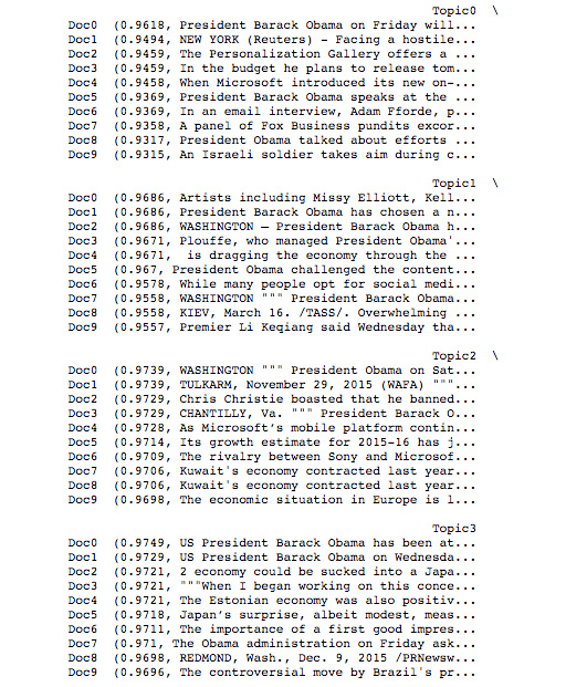
   Figure 7.41: The document-topic table using the four-topic LDA model

5. Display the results of the LDA model using pyLDAvis:

   lda4_plot = pyLDAvis.sklearn.prepare(lda4, clean_vec1, vectorizer1, R=10)

   pyLDAvis.display(lda4_plot)

   The plot is as follows:

Figure 7.42: A histogram and biplot describing the four-topic LDA model

Looking at the word-topic table, we see that the four topics found by this model align with the four topics specified in the original dataset. Those topics are Barack Obama, Palestine, Microsoft, and the economy. The question now is, why did the model built using four topics have a higher perplexity score than the model with three topics? That answer comes from the visualization produced in step 5. The biplot has circles of reasonable size, but two of those circles are quite close together, which suggests that those two topics, Microsoft and the economy, are very similar. In this case, the similarity actually makes intuitive sense. Microsoft is a major global company that impacts and is impacted by the economy. A next step, if we were to make one, would be to run the t-SNE plot to check whether the clusters in the t-SNE plot overlap. Let's now apply our knowledge of LDA to another dataset.

Activity 16: Latent Dirichlet Allocation and Health Tweets

In this activity, we apply LDA to the health tweets data loaded and cleaned in Activity 15, Loading and Cleaning Twitter Data. Remember to use the same notebook used in Activity 15, Loading and Cleaning Twitter Data. Once the steps have been executed, discuss the results of the model. Do these word groupings make sense?

For this activity, let's imagine that we are interested in acquiring a high-level understanding of the major public health topics. That is, what people are talking about in the world of health. We have collected some data that could shed light on this inquiry. The easiest way to identify the major topics in the dataset, as we have discussed, is topic modeling.

Here are the steps to complete the activity:

1. Specify the number_words, number_docs, and number_features variables.
2. Create a bag-of-words model and assign the feature names to another variable for use later on.
3. Identify the optimal number of topics.
4. Fit the LDA model using the optimal number of topics.
5. Create and print the word-topic table.
6. Print the document-topic table.
7. Create a biplot visualization.
8. Keep the notebook open for future modeling.

   The output will be as follows:

Figure 7.43: A histogram and biplot for the LDA model trained on health tweets

Note

The solution for this activity can be found on page 360.

Bag-of-Words Follow-Up

When running LDA models, the count vectorizer bag-of-words model was used, but that is not the only bag-of-words model. Term Frequency – Inverse Document Frequency (TF-IDF) is similar to the count vectorizer used in the LDA algorithm, except that instead of returning raw counts, TF-IDF returns a weight that reflects the importance of a given word to a document in the corpus. The key component of this weighting scheme is that there is a normalization component for how frequently a given word appears across the entire corpus. Consider the word have.

The word have may occur several times in a single document, suggesting that it could be important for isolating the topic of that document, but have will occur in many documents, if not most, in the corpus, potentially rendering it unless for isolating topics. Essentially, this scheme goes one step further than just returning the raw counts of the words in the document in an effort to initially identify words that may help identify abstract topics. The TF-IDF vectorizer is executed using sklearn via TfidfVectorizer.

Exercise 36: Creating a Bag-of-Words Using TF-IDF

In this exercise, we will create a bag-of-words using TF-IDF:

1. Run the TF-IDF vectorizer and print out the first few rows:

   vectorizer2 = sklearn.feature_extraction.text.TfidfVectorizer(

   analyzer="word",

   max_df=0.5,

   min_df=20,

   max_features=number_features,

   smooth_idf=False

   )

   clean_vec2 = vectorizer2.fit_transform(clean_sentences)

   print(clean_vec2[0])

   The output is as follows:

   

   Figure 7.44: Output of the TF-IDF vectorizer

2. Return the feature names, the actual words in the corpus dictionary, to use when analyzing the output. You recall that we did the same thing when we ran the CountVectorizer in Exercise 31, Creating Bag-of-Words Model Using the Count Vectorizer:

   feature_names_vec2 = vectorizer2.get_feature_names()

   feature_names_vec2

   A section of the output is as follows:

   ['abbas',

   'ability',

   'accelerate',

   'accept',

   'access',

   'accord',

   'account',

   'accused',

   'achieve',

   'acknowledge',

   'acquire',

   'acquisition',

   'across',

   'action',

   'activist',

   'activity',

   'actually',

Non-Negative Matrix Factorization

Unlike LDA, non-negative matrix factorization (NMF) is not a probabilistic model. It is instead, as the name implies, an approach involving linear algebra. Using matrix factorization as an approach to topic modeling was introduced by Daniel D. Lee and H. Sebastian Seung in 1999. The approach falls into the decomposition family of models that includes PCA, the modeling technique introduced in Chapter 4, An Introduction to Dimensionality Reduction & PCA.

The major differences between PCA and NMF are that PCA requires components to be orthogonal while allowing them to be either positive or negative. NMF requires matrix components be non-negative, which should make sense if you think of this requirement in the context of the data. Topics cannot be negatively related to documents and words cannot be negatively related to topics. If you are not convinced, try to interpret a negative weight associating a topic with a document. It would be something like, topic T makes up -30% of document D; but what does that even mean? It is nonsensical, so NMF has non-negative requirements for every part of matrix factorization.

Let's define the matrix to be factorized, call it X, as a term-document matrix where the rows are words and the columns are documents. Each element of matrix X is either the number of occurrences of word i (the row) in document j (the column) or some other quantification of the relationship between word i and document j. The matrix, X, is naturally a sparse matrix as most elements in the term-document matrix will be zero, since each document only contains a limited number of words. There will be more on creating this matrix and deriving the quantifications later:

Figure 7.45: The matrix factorization

The matrix factorization takes the form , where the two component matrices, W and H, represent the topics as collections of words and the topic weights for each document, respectively. More specifically, is a word by topic matrix, is a topic by document matrix, and, as stated earlier, is a word by document matrix. A nice way to think of this factorization is as a weighted sum of word groupings defining abstract topics. The equivalency symbol in the formula for the matrix factorization is an indicator that the factorization WH is an approximation and thus the product of those two matrices will not reproduce the original term-document matrix exactly. The goal, as it was with LDA, is to find the approximation that is closest to the original matrix. Like X, both W and H are sparse matrices as each topic is only related to a few words and each document is a mixture of only a small number of topics – one topic in many cases.

Frobenius Norm

The goal of solving NMF is the same as that of LDA: find the best approximation. To measure the distance between the input matrix and the approximation, NMF can use virtually any distance measure, but the standard is the Frobenius norm, also known as the Euclidean norm. The Frobenius norm is the sum of the element-wise squared errors mathematically expressed as .

With the measure of distance selected, the next step is defining the objective function. The minimization of the Frobenius norm will return the best approximation of the original term-document matrix and thus the most reasonable topics. Note that the objective function is minimized with respect to W and H so that both matrices are non-negative. It is expressed as .

Multiplicative Update

The optimization algorithm used to solve NMF by Lee and Seung in their 1999 paper is the Multiplicative Update algorithm and it is still one of the most commonly used solutions. It will be implemented in the exercises and activities later in the chapter. The update rules, for both W and H, are derived by expanding the objective function and taking the partial derivatives with respect to W and H. The derivatives are not difficult but do require fairly extensive linear algebra knowledge and are time-consuming, so let's skip the derivatives and just state the updates. Note that, in the update rules, i is the current iteration and T means the transpose of the matrix. The first update rule is as follows:

Figure 7.46: First update rule

The second update rule is as follows:

Figure 7.47: Second update rule

W and H are updated iteratively until the algorithm converges. The objective function can also be shown to be non-increasing. That is, with each iterative update of W and H, the objective function gets closer to the minimum. Note that the multiplicative update optimizer, if the update rules are reorganized, is a rescaled gradient descent algorithm.

The final component of building a successful NMF algorithm is initializing the W and H component matrices so that the multiplicative update works quickly. A popular approach to initializing matrices is Singular Value Decomposition (SVD), which is a generalization of Eigen decomposition. In the implementation of NMF done in the forthcoming exercises, the matrices are initialized via non-negative Double Singular Value Decomposition, which is basically a more advanced version of SVD that is strictly non-negative. The full details of these initialization algorithms are not important to understanding NMF. Just note that initialization algorithms are used as a starting point for the optimization algorithms and can drastically speed up convergence.

Exercise 37: Non-negative Matrix Factorization

In this exercise, we fit the NMF algorithm and output the same two result tables we did with LDA previously. Those tables are the word-topic table, which shows the top-10 words associated with each topic, and the document-topic table, which shows the top-10 documents associated with each topic. There are two additional parameters in the NMF algorithm function that we have not previously discussed, which are alpha and l1_ratio. If an overfit model is of concern, these parameters control how (l1_ratio) and the extent to which (alpha) regularization is applied to the objective function. More details can be found in the documentation for the scikit-learn library (https://scikit-learn.org/stable/modules/generated/sklearn.decomposition.NMF.html):

1. Define the NMF model and call the fit function using the output of the TF-IDF vectorizer:

   nmf = sklearn.decomposition.NMF(

   n_components=4,

   init="nndsvda",

   solver="mu",

   beta_loss="frobenius",

   random_state=0,

   alpha=0.1,

   l1_ratio=0.5

   )

   nmf.fit(clean_vec2)

   The output is as follows:

   

   Figure 7.48: Defining the NMF model

2. Run the get_topics functions to produce the two output tables:

   W_df, H_df = get_topics(

   mod=nmf,

   vec=clean_vec2,

   names=feature_names_vec2,

   docs=raw,

   ndocs=number_docs,

   nwords=number_words

   )

3. Print the W table:

   print(W_df)

   The output is as follows:

   

   Figure 7.49: The word-topic table containing probabilities

4. Print the H table:

   print(H_df)

Figure 7.50: The document-topic table containing probabilities

The word-topic table contains word groupings that suggest the same abstract topics that the four-topic LDA model produced in Exercise 35, Trying four topics. However, the interesting part of the comparison is that some of the individual words contained in these groupings are new or in a new place in the grouping. This is not surprising given that the methodologies are distinct. Given the alignment with the topics specified in the original dataset, we have shown that both of these methodologies are effective tools for extracting the underlying topic structure of the corpus.

Exercise 38: Visualizing NMF

The purpose of this exercise is to visualize the results of NMF. Visualizing the results gives insights into the distinctness of the topics and the prevalence of each topic in the corpus. In this exercise, we do the visualizing using t-SNE, which was discussed fully in Chapter 6, t-Distributed Stochastic Neighbor Embedding (t-SNE):

1. Run transform on the cleaned data to get the topic-document allocations. Print both the shape and an example of the data:

   nmf_transform = nmf.transform(clean_vec2)

   print(nmf_transform.shape)

   print(nmf_transform)

   The output is as follows:

   

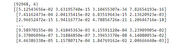
   Figure 7.51: Shape and example of data

2. Run the plot_tsne function to fit a t-SNE model and plot the results:

   plot_tsne(data=nmf_transform, threshold=0)

   The plot looks as follows:

Figure 7.52: t-SNE plot with metrics summarizing the topic distribution across the corpus

The t-SNE plot, with no threshold specified, shows some topic overlap and a clear discrepancy in the topic frequency across the corpus. These two facts explain why, when using perplexity, the optimal number of topics is three. There seems to be some correlation between topics that the model can't fully accommodate. Even with the correlation between topics, the model is finding the topics it should when the number of topics is set to four.

To recap, NMF is a non-probabilistic topic model that seeks to answer the same question LDA is trying to answer. It uses a popular concept of linear algebra known as matrix factorization, which is the process of breaking a large and intractable matrix down into smaller and more easily interpretable matrices that can be leveraged to answer many questions about the data. Remember that the non-negative requirement is not rooted in mathematics, but in the data itself. It does not make sense for the components of any documents to be negative. In many cases, NMF does not perform as well as LDA, because LDA incorporates prior distributions that add an extra layer of information to help inform the topic word groupings. However, we know that there are cases, especially when the topics are highly correlated, when NMF is the better performer. One of those cases was the headline data on which all the exercises were based.

Activity 17: Non-Negative Matrix Factorization

This activity is the summation of the topic modeling analysis done on the health Twitter data loaded and cleaned in activity one, and on which LDA was done in activity two. The execution of NMF is straightforward and requires limited coding, so I suggest taking this opportunity to play with the parameters of the model while thinking about the limitations and benefits of NMF.

Here are the steps to complete the activity:

1. Create the appropriate bag-of-words model and output the feature names as another variable.
2. Define and fit the NMF algorithm using the number of topics (n_components) value from activity two.
3. Get the topic-document and word-topic result tables. Take a few minutes to explore the word groupings and try to define the abstract topics. Can you quantify the meanings of the word groupings? Do the word groupings make sense? Are the results similar to those produced using LDA?
4. Adjust the model parameters and rerun step 3 and step 4. How do the results change?

   The output will be as follows:

Figure 7.53: The word-topic table with probabilities

Note

The solution for this activity can be found on page 364.

Summary

When faced with the task of extracting information from an as yet unseen large collection of documents, topic modeling is a great approach, as it provides insights into the underlying structure of the documents. That is, topic models find word groupings using proximity, not context. In this chapter, we have learned how to apply two of the most common and most effective topic modeling algorithms: latent Dirichlet allocation and non-negative matrix factorization. We should now feel comfortable cleaning raw text documents using several different techniques; techniques that can be utilized in many other modeling scenarios. We continued by learning how to convert the cleaned corpus into the appropriate data structure of per-document raw word counts or word weights by applying bag-of-words models. The main focus of the chapter was fitting the two topic models, including optimizing the number of topics, converting the output to easy-to-interpret tables, and visualizing the results. With this information, you should be able to apply fully functioning topic models to derive value and insights for your business.

In the next chapter, we will change directions entirely. We will deep dive into market basket analysis.