Chapter 5

Data Comparison Methods

Learning Objectives

By the end of this chapter, you will be able to:

• Create hashes of data
• Create image signatures
• Compare image datasets
• Perform factor analysis to isolate latent variables
• Compare surveys and other datasets using factor analysis

In this chapter, we will have a look at different data comparison methods.

Introduction

Unsupervised learning is concerned with analyzing the structure of data to draw useful conclusions. In this chapter, we will examine methods that enable us to use the structure of data to compare datasets. The major methods we will look at are hash functions, analytic signatures, and latent variable models.

Hash Functions

Imagine that you want to send an R script to your friend. However, you and your friend have been having technical problems with your files – maybe your computers have been infected by malware, or maybe a hacker is tampering with your files. So, you need a way to ensure that your script is sent intact to your friend, without being corrupted or changed. One way to check that files are intact is to use hash functions.

A hash function can create something like a fingerprint for data. What we mean by a fingerprint is something that is small and easy to check that enables us to verify whether the data has the identity we think it should have. So, after you create the script you want to send, you apply your hash function to the script and get its fingerprint. Then, your friend can use the same hash function on the file after it is received and check to make sure the fingerprints match. If the fingerprint of the file that was sent matches the fingerprint of the file that was received, then the two files should be the same, meaning that the file was sent intact. The following exercise shows how to create and use a simple hash function.

Exercise 29: Creating and Using a Hash Function

In this exercise, we will create and use a hash function:

1. Specify the data on which you need to use the hash function. We have been exploring the scenario of an R script that you want to send. Here is an example of a simple R script:

   string_to_hash<-"print('Take the cake')"

   Here, we have a script that prints the string Take the cake. We have saved it as a variable called string_to_hash.

2. Specify the total number of possible hash values. Our goal is to create a fingerprint for our script. We need to specify the total number of possible fingerprints that we will allow to exist. We want to specify a number that is low enough to work with easily, but high enough that there is not much likelihood of different scripts having the same fingerprint by coincidence. Here, we will use 10,000:

   total_possible_hashes<-10000

3. Convert the script (currently a string) to numeric values. Hash functions are usually arithmetic, so we will need to be working with numbers instead of strings. Luckily, R has a built-in function that can accomplish this for us:

   numeric<-utf8ToInt(string_to_hash)

   This has converted each of the characters in our script to an integer, based on each character's encoding in the UTF-8 encoding scheme. We can see the result by printing to the console:

   print(numeric)

   The output is as follows:

   [1] 112 114 105 110 116 40 39 84 97 107 101 32 116 104 101 32 99 97 107[20] 101 39 41

4. Apply our hashing function. We will use the following function to generate our final hash, or in other words, the fingerprint of the script:

   hash<-sum((numeric+123)^2) %% total_possible_hashes

   After running this line in R, we find that the final value of hash is 2702. Since we have used the modulo operator (%% in R), the value of hash will always be between 0 and 10,000.

The simple function we used to convert a numeric vector to a final hash value is not the only possible hash function. Experts have designed many such functions with varying levels of sophistication. There is a long list of properties that good hash functions are supposed to have. One of the most important of these properties is collision resistance, which means that it is difficult to find two datasets that yield the same hash.

Exercise 30: Verifying Our Hash Function

In this exercise, we will verify that our hash function enables us to effectively compare different data by checking that different messages produce different hashes. The outcome of this exercise will be hash functions of different messages that we will compare to verify that different messages produce different hashes:

1. Create a function that performs hashing for us. We will put the code that we introduced in the preceding exercise together into one function:

   get_hash<-function(string_to_hash, total_possible_hashes){

   numeric<-utf8ToInt(string_to_hash)

   hash<-sum((numeric+123)^2) %% total_possible_hashes

   return(hash)

   }

   This function takes the string we want to hash and the total number of possible hashes, then applies the same hashing calculation we used in the previous exercise to calculate a hash, and then returns that hash value.

2. Compare hashes of different inputs. We can compare the hashes that are returned from different inputs as follows:

   script_1<-"print('Take the cake')"

   script_2<-"print('Make the cake')"

   script_3<-"print('Take the rake')"

   script_4<-"print('Take the towel')"

   Here, we have four different strings, expressing different messages. We can see the value of their hashes as follows:

   print(get_hash(script_1,10000))

   print(get_hash(script_2,10000))

   print(get_hash(script_3,10000))

   print(get_hash(script_4,10000))

   The first script returns the hash 2702, as we found in the preceding exercise. The second script, even though it is only differs from the first script by one character, returns the hash 9853, and the third script, also differing by only one character from the first script, returns the hash 9587. The final script returns the hash 5920. Though these four scripts have substantial similarities, they have different fingerprints that we can use to compare them and distinguish them.

These hashes are useful for you and the recipient of your message to verify that your script was sent intact without tampering. When you send the script, you can tell your friend to make sure that the hash of the script is 2702. If the hash of the script your friend receives is not 2702, then your friend can conclude that the script was tampered with between being sent and being received. If your friend can reliably detect whether a file was corrupted, then you can avoid spreading malware or arguing with your friend over miscommunication.

Software that is distributed online is sometimes distributed with a hash value that users can use to check for file corruption. For this purpose, professionals use hash functions that are more advanced than the simple function presented in the preceding exercises. One of the hash functions that professionals use is called MD5, which can be applied very easily in R using the digest package:

install.packages('digest')

library(digest)

print(digest(string_to_hash,algo='md5'))

The output is as follows:

[1] "a3d9d1d7037a02d01526bfe25d1b7126"

Here, we can see the MD5 hash of our simple R script. You can feel free to try out MD5 hashes of other data as well to compare the results.

Analytic Signatures

In Chapter 4, Dimension Reduction, we discussed dimension reduction – methods that enable us to express data succinctly in ways that give us insights into the data. A hash function, discussed previously, is yet another way to accomplish dimension reduction. Hash functions are effective for many purposes, including the file verification use case we discussed. In that scenario, we were interested in determining whether two scripts were exactly the same or not. Even a slight difference in data, such as changing the word "take" to "make," had the potential to completely corrupt the intended message, so exactness was required.

In other cases, we may want to make meaningful comparisons between different datasets without requiring the exact identity of the two datasets being compared. Consider the case of detecting copyright violations. Suppose that a website hosts images from its users. It wants to ensure that users are not submitting images that are protected by copyright. So, every time it receives an upload, it wants to check whether that upload is the same as any of the images in a large database of copyrighted images.

It is not sufficient to check whether images are exactly the same, since unscrupulous uploaders may make slight alterations and attempt to upload anyway. For example, they might change the color of one pixel, or crop the image very slightly, or compress it to be larger or smaller than the original. Even with these slight alterations, the images would still violate copyright laws. A hash function that checked for exact identity would fail to recognize these copyright violations. So, the image hosting site will want to check whether there is any underlying structure in the data representing the two pictures that is substantially similar.

We mentioned that hash functions created something that's like a fingerprint for data. Fingerprints should be exactly the same each time they are observed, and even if two fingerprints are similar in most ways, we will not regard them as matching each other unless they match completely.

Instead of a fingerprint, in this case we need something more like a signature. Each time you sign your name, your signature should look more or less the same. But, there will be small differences in each signature, even when signed by the same person and even when attempting to match previous signatures. In order to verify whether a signature matches, we need to check for substantial similarity but not perfect identity. The code we present here will show how to encode any image of any size in a small and robust encoding that enables quick and accurate approximate comparisons between datasets. This method for encoding image data can be referred to as creating an analytic signature.

Our method for creating a signature for an image will proceed as follows. First, we will divide our image into a 10x10 grid. We will then measure the brightness of each section of this grid. After that, we will compare the brightness of each section to the brightness of its neighbors. The final signature will consist of a vector of comparisons between each grid section and each of its neighbors. This signature method was invented by Wong, Bern, and Goldberg, who published it in a paper called An Image Signature for Any Kind of Image.

Before we create an analytic signature, we will need to do some data preparation, as outlined in the next exercise.

Exercise 31: Perform the Data Preparation for Creating an Analytic Signature for an Image

In this exercise, we will perform the data preparation for creating an analytic signature for a photo of the Alamo.

Note

For all the exercises and activities where we are importing external CSV files or images, go to RStudio-> Session-> Set Working Directory-> To Source File Location. You can see in the console that the path is set automatically.

1. First, we will need to configure R to be able to read in and work with our image data. We will need to install the imager package. You can install this package by executing install.packages('imager') in the R console, and then you can load it by running library('imager') in the console.
2. Next, we will need to read in the data. We will be working with this photo of the Alamo in our example:
   

   Figure 5.1: Alamo image

   First, download this to your computer from https://github.com/TrainingByPackt/Applied-Unsupervised-Learning-with-R/Lesson05/Exercise31/alamo.jpg and save it as alamo.jpg. Make sure that it is saved in R's working directory. If it is not in R's working directory, then change R's working directory using the setwd() function. Then, you can load this image into a variable called im (short for image) as follows:

   filepath<-'alamo.jpg'

   im <- imager::load.image(file =filepath)

   The rest of the code we will explore will use this image called im. Here, we have loaded a photo of the Alamo into im. However, you can run the rest of the code on any image, simply by saving the image to your working directory and specifying its path in the filepath variable.

3. The signature we are developing is meant to be used for grayscale images. So, we will convert this image to grayscale by using functions in the imager package:

   im<-imager::rm.alpha(im)

   im<-imager::grayscale(im)

   im<-imager::imsplit(im,axis = "x", nb = 10)

   The second line of this code is the conversion to grayscale. The last line performs a split of the image into 10 equal sections.

4. The following code creates an empty matrix that we will fill with information about each section of our 10x10 grid:

   matrix <- matrix(nrow = 10, ncol = 10)

   Next, we will run the following loop. The first line of this loop uses the imsplit command. This command was also used earlier to split the x-axis into 10 equal parts. This time, for each of the 10 x-axis splits, we will do a split along the yaxis, also splitting it into 10 equal parts:

   for (i in 1:10) {

   is <- imager::imsplit(im = im[[i]], axis = "y", nb = 10)

   for (j in 1:10) {

   matrix[j,i] <- mean(is[[j]])

   }

   }

   After splitting along the y axis, the matrix is updated with mean(is[[j]]). This is a measure of the mean brightness of the selected section.

   The result of this code is a 10x10 matrix, where the i-j element contains the average brightness of the i-j section of the original photo.

   If you print this matrix, you can see the brightness numbers for each section of the photo:

   print(matrix)

   The output should look like the following:

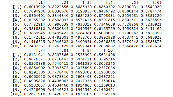
Figure 5.2: Screenshot of the output matrix

You can compare these brightness numbers to the appearance of the original photo.

We could stop here, since we have generated a compressed encoding of a complex dataset. However, we can take some further steps to make this encoding more useful.

One thing we can do is create a brightnesscomparison function. The purpose of this function is to compare the relative brightness of two different sections of an image. Eventually, we will compare all of the different sections of each image we analyze. Our final fingerprint will consist of many such brightness comparisons. The purpose of this exercise is to create the brightness comparison function that will eventually enable us to create the final fingerprint.

Please note, this exercise is built on top of the previous exercise, meaning that you should run all of the code in the previous exercise before you run the code in this exercise.

Exercise 32: Creating a Brightness Comparison Function

1. In this function, we pass two arguments, x and y: each argument represents the brightness of a particular section of the picture. If x and y are quite similar (less than 10% different), then we say that they are essentially the same and we return 0, indicating approximately 0 difference in brightness. If x is more than 10% greater than y, we return 1, indicating that x is brighter than y, and if x is more than 10% smaller than y, we return -1, indicating that x is less bright than y.
2. Create the brightness comparison function. The code for the brightnesscomparison function is as follows:

   brightnesscomparison<-function(x,y){

   compared<-0

   if(abs(x/y-1)>0.1){

   if(x>y){

   compared<-1

   }

   if(x<y){

   compared<-(-1)

   }

   }

   return(compared)

   }

3. We can use this function to compare two sections of the 10x10 grid we formed for our picture. For example, to find the brightness comparison of a section with the section that is directly to its left, we can execute the following code:

   i<-5

   j<-5

   left<-brightnesscomparison(matrix[i,j-1],matrix[i,j])

   Here, we looked at the 5th row and 5th column of our matrix. We compared this section to the section directly to the left of it – the 5th row and 4th column, which we accessed by specifying j-1.

4. Use the brightness comparison function to compare an image section to its neighbor above it. We could do an analogous operation to compare this section to the section above it:

   i<-5

   j<-5

   top<-brightnesscomparison(matrix[i-1,j],matrix[i,j])

Here, top is a comparison of the brightness of section 5, 5 with the section immediately above it, which we accessed by specifying i-1.

The important outputs of this exercise are the values of top and left, which are both comparisons of an image section to other, neighboring sections. In this case, left is equal to zero, meaning that the image section we selected has about the same brightness as the image section to its left. Also, top is equal to 1, meaning that the section directly above the section we selected is brighter than the section we selected.

In the next exercise, we will create a neighborcomparison function. This function takes every section of our 10x10 grid and compares the brightness of that section to its neighbors. These neighbors include the left neighbor, whose brightness we compared a moment ago, and also the top neighbor. Altogether, there are eight neighbors for each section of our picture (top, bottom, left, right, top-left, top-right, bottom-left, and bottom-right). The reason we will want this neighbor comparison function is because it will make it very easy for us to get our final analytic signature.

Please note that this exercise builds on the previous exercises, and you should run all of the previous code before running this code.

Exercise 33: Creating a Function to Compare Image Sections to All of the Neighboring Sections

In this exercise, we will create a neighborcomparison function to compare image sections to all other neighboring sections. To do this, perform the following steps:

1. Create a function that compares an image section to its neighbor on the left. We did this in the previous exercise. For any image section, we can compare its brightness to the brightness of its neighbor on the left as follows:

   i<-5

   j<-5

   left<-brightnesscomparison(matrix[i,j-1],matrix[i,j])

2. Create a function that compares an image section to its neighbor on top. We did this in the previous exercise. For any image section, we can compare its brightness to the brightness of its neighbor above it as follows:

   i<-5

   j<-5

   top<-brightnesscomparison(matrix[i-1,j],matrix[i,j])

3. If you look at Step 1 and Step 2, you can start to notice the pattern in these neighbor comparisons. To compare an image section to the section on its left, we need to access the part of the matrix at index j-1. To compare an image section to the section on its right, we need to access the part of the matrix at index j+1. To compare an image section to the section above it, we need to access the part of the matrix at index i-1. To compare an image section to the section below it, we need to access the part of the matrix at index i+1.

   So, we will have comparisons of each image section to each of its neighbors, above, below, left, and right. The following code shows the comparisons we will make in addition to the top and left comparisons made in Step 1 and Step 2:

   i<-5

   j<-5

   top_left<-brightnesscomparison(matrix[i-1,j-1], matrix[i,j])

   bottom_left<-brightnesscomparison(matrix[i+1,j-1],matrix[i,j])

   top_right<-brightnesscomparison(matrix[i-1,j+1],matrix[i,j])

   right<-brightnesscomparison(matrix[i,j+1],matrix[i,j])

   bottom_right<-brightnesscomparison(matrix[i+1,j+1],matrix[i,j])

   bottom<-brightnesscomparison(matrix[i+1,j],matrix[i,j])

4. Initialize a vector that will contain the final comparison of a section to each of its neighbors:

   comparison<-NULL

   We will use this comparison vector to store all of the neighbor comparisons that we eventually generate. It will consist of comparisons of an image section to each of its neighbors.

5. In steps 1-4, we have shown the individual parts of the neighbor comparison function. In this step, we will combine them. The neighbor comparison function that you can see takes an image matrix as an argument, and also i and j values, specifying which part of the image matrix we are focusing on. The function uses the code we wrote for the top and left comparisons, and also adds other comparisons for other neighbors, such as top_left, which compares an image brightness level with the image brightness of the section above and to the left. Altogether, each image section should have eight neighbors: top-left, top, top-right, left, right, bottom-left, bottom, and bottom-right. In this step, we will do each of these eight comparisons and store them in the comparison vector. Finally, there is a return statement that returns all of the comparisons together.

   Here is the function we can use to get all of the neighbor comparisons:

   neighborcomparison<-function(mat,i,j){

   comparison<-NULL

   top_left<-0

   if(i>1 & j>1){

   top_left<-brightnesscomparison(mat[i-1,j-1],mat[i,j])

   }

   left<-0

   if(j>1){

   left<-brightnesscomparison(mat[i,j-1],mat[i,j])

   }

   bottom_left<-0

   if(j>1 & i<nrow(mat)){

   bottom_left<-brightnesscomparison(mat[i+1,j-1],mat[i,j])

   }

   top_right<-0

   if(i>1 & j<nrow(mat)){

   top_right<-brightnesscomparison(mat[i-1,j+1],mat[i,j])

   }

   right<-0

   if(j<ncol(mat)){

   right<-brightnesscomparison(mat[i,j+1],mat[i,j])

   }

   bottom_right<-0

   if(i<nrow(mat) & j<ncol(mat)){

   bottom_right<-brightnesscomparison(mat[i+1,j+1],mat[i,j])

   }

   top<-0

   if(i>1){

   top<-brightnesscomparison(mat[i-1,j],mat[i,j])

   }

   bottom<-0

   if(i<nrow(mat)){

   bottom<-brightnesscomparison(mat[i+1,j],mat[i,j])

   }

   comparison<-c(top_left,left,bottom_left,bottom,bottom_right,right,top_right,top)

   return(comparison)

   }

This function returns a vector with eight elements: one for each of the neighbors of a particular section of our grid. You may have noticed that some sections of the 10x10 grid do not appear to have eight neighbors. For example, the 1-1 element of the 10x10 grid has a neighbor below it, but does not have a neighbor above it. For grid locations that do not have particular neighbors, we say that their brightness comparison is 0 for that neighbor. This decreases the level of complexity in creating and interpreting the brightness comparisons.

The final output is a vector called comparison, which contains comparisons of brightness levels between an image section and each of its eight neighbors.

In the next exercise, we will finish creating our analytic signature. The analytic signature for each image will consist of comparisons of each image section with each of its eight neighbors. We will use two nested for loops to iterate through every section of our 10x10 grid. The expected output of this exercise will be a function that generates an analytic signature for an image.

Exercise 34: Creating a Function that Generates an Analytic Signature for an Image

In this exercise, we will create a function that generates an analytic signature for an image. To do this, perform the following steps:

1. We begin by creating a signature variable and initializing it with a NULL value:

   signature<-NULL

   This signature variable will store the complete signature when we have finished.

2. Now we can loop through our grid. For each section of the grid, we add eight new elements to the signature. The elements we add are the outputs of the neighborcomparison function we introduced earlier:

   for (i in 1:nrow(matrix)){

   for (j in 1:ncol(matrix)){

   signature<-c(signature,neighborcomparison(matrix,i,j))

   }

   }

   We can see what our fingerprint looks like by running print(signature) in the console. It is a vector of 800 values, all of which are equal to either 0 (indicating similar brightness or no neighbor), 1 (indicating that a section is more bright than its neighbor), or -1 (indicating that a section is less bright than its neighbor).

3. Put Step 1 and Step 2 together in a function that can generate a signature for any image matrix:

   get_signature<-function(matrix){

   signature<-NULL

   for (i in 1:nrow(matrix)){

   for (j in 1:ncol(matrix)){

   signature<-c(signature,neighborcomparison(matrix,i,j))

   }

   }

   return(signature)

   }

   This code defines a function called get_signature, and it uses the code from Step 1 and Step 2 to get that signature. We can call this function using the image matrix we created earlier.

4. Since we are going to create more signatures later, we will save this signature to a variable that refers to what it is a signature of. In this case, we will call it building_signature since it is a signature of an image of a building. We can do this as follows:

   building_signature<-get_signature(matrix)

   building_signature

   The output is as follows:

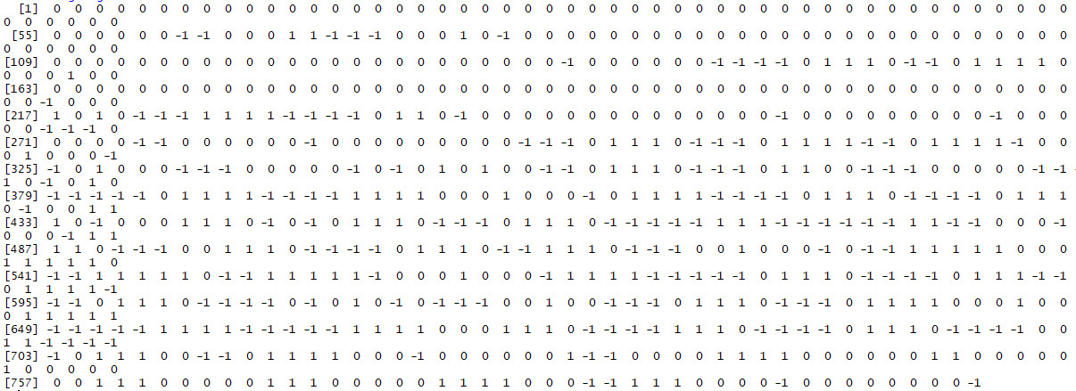
Figure: 5.3: Matrix of building_signature

The vector stored in building_signature is the final output of this exercise, and it is the image signature we have been trying to develop throughout this chapter.

This signature is meant to be like a human's handwritten signature: small and apparently similar to other signatures, but sufficiently unique to enable us to distinguish it from millions of other existing signatures.

We can check the robustness of the signature solution we have found by reading in a completely different image and comparing the resulting signatures. This is the scenario for the following activity.

Activity 11: Creating an Image Signature for a Photograph of a Person

Let's try to create an image fingerprint for this image, a photograph of the great Jorge Luis Borges.

To accomplish this activity, you can follow all of the steps we have followed so far in this chapter. The following steps will outline this process for you. Remember that in our previous image signature exercise, we used a 10x10 matrix of brightness measurements. However, a 10x10 matrix may be inappropriate for some situations, for example, if the image we are working with is particularly small, or if we have data storage constraints, or if we expect higher accuracy with a different matrix size. So, in the following activity, we will also calculate a signature using a 9x9 matrix:

Note

This can be performed on any given matrix size. It could be a 5x5 matrix for data storage purposes or a 20x20 matrix for accurate signatures.

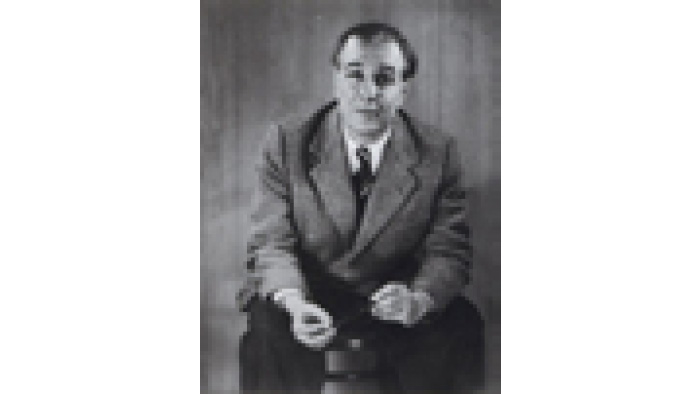
Figure 5.4: Jorge Luis Borges image

These steps will help us complete the activity:

1. Load the image into your R working directory. Save it to a variable called im.
2. Convert your image to grayscale and split it into 100 sections.
3. Create a matrix of brightness values.
4. Create a signature using the get_signature function we created earlier. Save the signature of the Borges image as borges_signature.

   Note

   The solution for this activity can be found on page 227.

The final output of this activity is the borges_signature variable, which is the analytic signature of the Borges photo. Additionally, we have created the borges_signature_ninebynine variable, which is also an analytic signature, but based on a 9x9 rather than a 10x10 matrix. We can use either of them in our analysis, but we will use the borges_signature variable. If you have completed all of the exercises and activities so far, then you should have two analytic signatures: one called building_signature, and one called borges_signature.

Comparison of Signatures

Next, we can compare these two signatures, to see whether they have mapped our different images to different signature values.

You can compare the signatures with one simple line of R code as follows:

comparison<-mean(abs(borges_signature-building_signature))

This comparison takes the absolute value of the difference between each element of the two signatures, and then calculates the mean of those values. If two signatures are identical, then this difference will be 0. The larger the value of comparison, the more different the two images are.

In this case, the value of comparison is 0.644, indicating that on average, the corresponding signature entries are about 0.644 apart. This difference is substantial for a dataset where the values only range between 1 and -1. So we see that our method for creating signatures has created very different signatures for very different images, as we would expect.

Now, we can calculate a signature for an image that is very similar to our original image, but not identical:

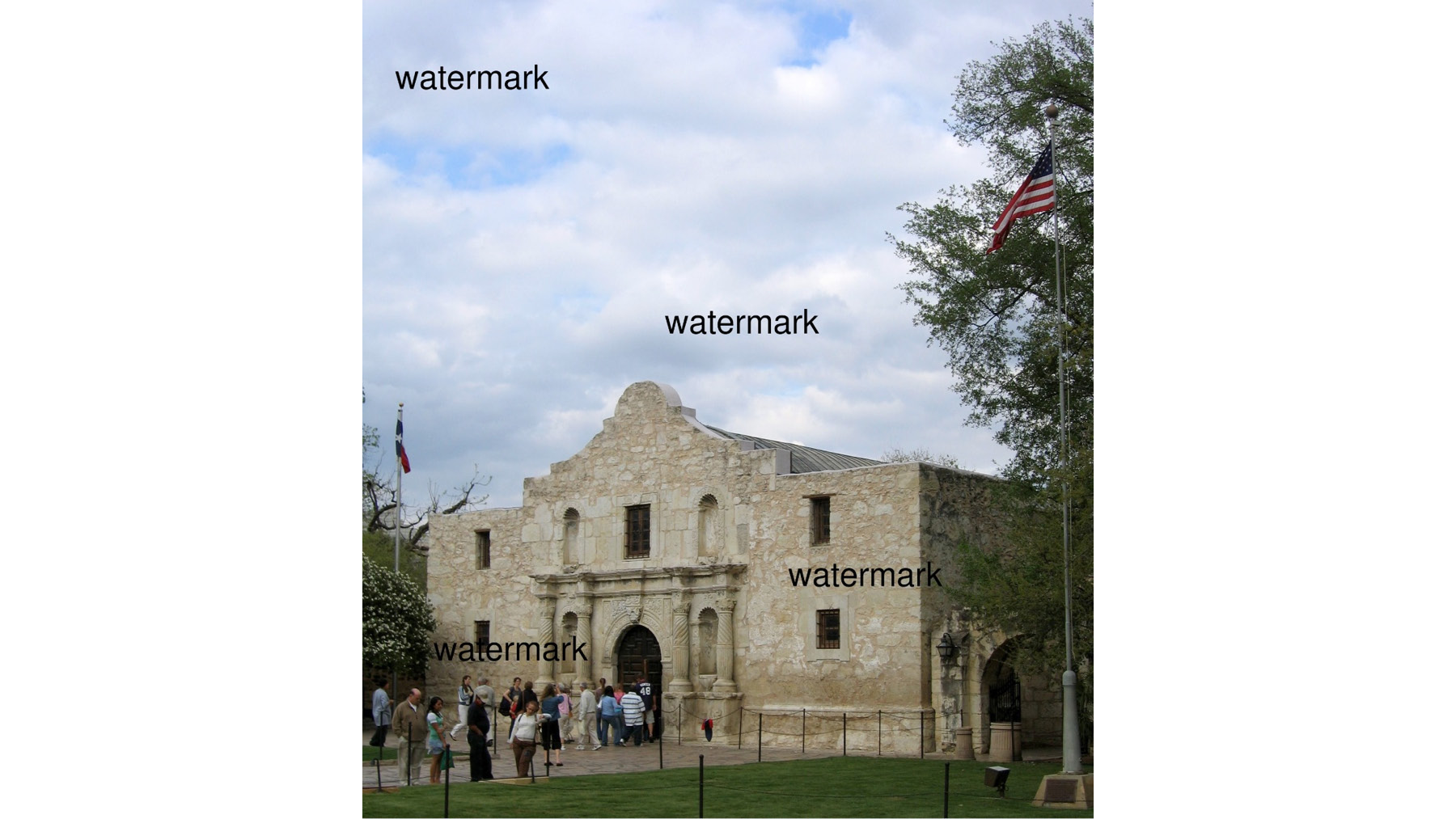
Figure 5.5: Alamo_marked image

To obtain this image, I started with the original Alamo image, and I added the word watermark in four places, simulating what someone might do to alter an image. Naive copyright detection software might be fooled by this watermark, since the image is now different from the original. Our analytic signature method should not be so naive. We will accomplish this in the following activity.

Activity 12: Creating an Image Signature for the Watermarked Image

In this activity, we will create an image signature for the watermarked image:

1. Load the image into your R working directory. Save it to a variable called im.
2. Convert your image to grayscale and split it into 100 sections.
3. Create a matrix of brightness values.
4. Create a signature using the get_signature function we created earlier. Save the signature of the Alamo image as watermarked_signature.
5. Compare the signature of the watermarked image to the signature of the original image to determine whether the signature method can tell the images apart.

   The output will be as follows:

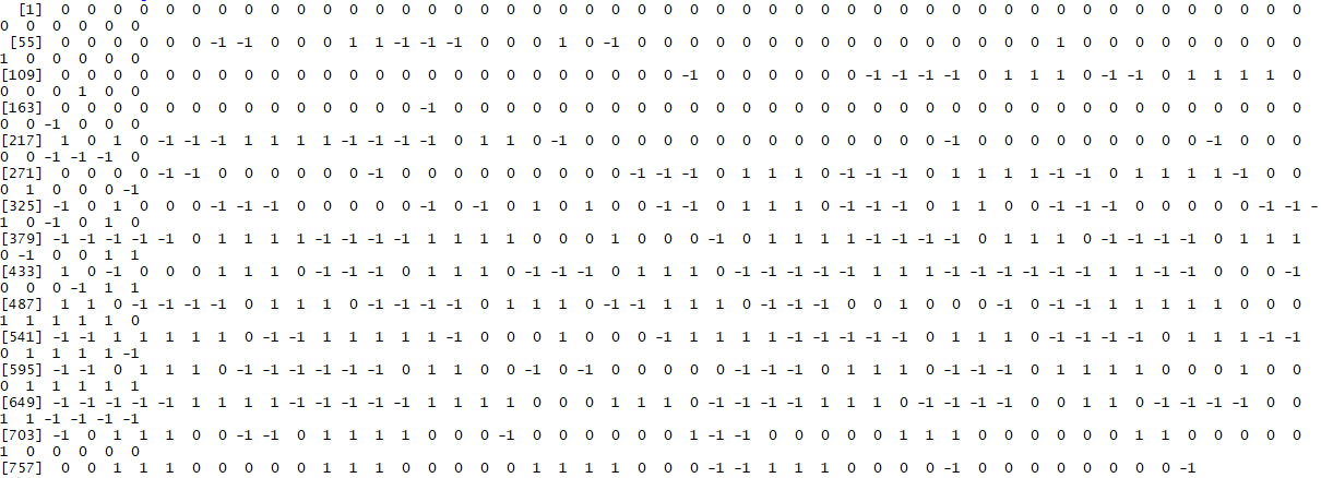
Figure 5.6: Expected signature of watermarked image

Note

The solution for this activity can be found on page 230.

In order to detect copyright violations, we can calculate signatures for every copyrighted image in a database. Then, for every newly uploaded image, we compare the signature of the newly uploaded image to the signatures in the database. If any of the copyrighted images have a signature that is identical to or substantially close to the signature of the new upload, we flag them as potential matches that need further investigation. Comparing signatures can be much faster than comparing original images, and it has the advantage of being robust to small changes such as watermarking.

The signature method we just performed is a way to encode data to enable comparisons between different datasets. There are many other encoding methods, including some that use neural networks. Each encoding method will have some of its own unique characteristics, but they will all share some common features: they will all try to return compressed data that enables easy and accurate comparison between datasets.

Applying Other Unsupervised Learning Methods to Analytic Signatures

So far, we have only used hashes and analytic signatures to compare two images or four short strings. However, there is no limit to the unsupervised learning methods that can be applied to hashes or analytic signatures. Creating analytic signatures for a set of images can be the first step of an in-depth analysis rather than the last step. After creating analytic signatures for a set of images, we can attempt the following unsupervised learning approaches:

• Clustering: We can apply any of the clustering methods discussed in the first two chapters to datasets consisting of analytic signatures. This could enable us to find groups of images that all tend to resemble each other, perhaps because they are photographs of the same type of object. Please see the first two chapters for more information about clustering methods.
• Anomaly detection: We can apply the anomaly detection methods described in Chapter 6, Anomaly Detection, to datasets that consist of analytic signatures. This will enable us to find images that are very different from the rest of the images in the dataset.

Latent Variable Models – Factor Analysis

This section will cover latent variable models. Latent variable models attempt to express data in terms of a small number of variables that are hidden or latent. By finding the latent variables that correspond to a dataset, we can better understand the data and potentially even understand where it came from or how it was generated.

Consider students receiving grades in a wide variety of classes, from math to music to foreign languages to chemistry. Psychologists or educators may be interested in using this data to better understand human intelligence. There are several different theories of intelligence that researchers might want to test in the data, for example:

• Theory 1: There are two different types of intelligence, and people who possess one type will excel in one set of classes, while people who possess the other type will excel in other classes.
• Theory 2: There is only one type of intelligence, and people who possess it will excel at all types of classes, and people who do not possess it will not.
• Theory 3: People may be highly intelligent when judged by the standards of one or a few of the classes they are taking, but not intelligent when judged by other standards, and every person will have a different set of classes at which they excel.

Each of these theories is expressing a notion of latent variables. The data only contains student grades, which could be a manifestation of intelligence but are not a direct measure of intelligence itself. The theories express ways that different kinds of intelligence affect grades in a latent way. Even though we do not know which theory is true, we can use tools of unsupervised learning to understand the structure of the data and which theory fits the data best.

Anyone who remembers being a student is probably fed up with people evaluating their intelligence. So, we will use a slightly different example. Instead of evaluating intelligence, we will evaluate personality. Instead of looking for a right brain and a left brain, we will look for different features of people's personalities. But we will take the same approach – using latent variables to identify whether complex data can be explained by some small number of factors.

In order to prepare for our analysis, we will need to install and load the right packages. The next exercise will cover how to load the packages that will be necessary for factor analysis.

Exercise 35: Preparing for Factor Analysis

In this exercise, we will prepare the data for factor analysis:

1. Install the necessary packages:

   install.packages('psych')

   install.packages('GPArotation')

   install.packages('qgraph')

2. Then, you can run the following lines to load them into your R workspace:

   library(psych)

   library(GPArotation)

   library(qgraph)

3. Next, load the data. The data we will use is a record of 500 responses to a personality test called the "Revised NEO Personality Inventory". The dataset is included in the R package called qgraph. To begin, read the data into your R workspace. This code will allow you to access it as a variable called big5:

   data(big5)

4. You can see the top section of the data by running the following line in the R console:

   print(head(big5))

   The output is as follows:

   

   Figure 5.7: Top section of the data

5. You can see the number of rows and columns of your data as follows:

   print(nrow(big5))

   The output is as follows:

   500

   To check the columns, execute the following:

   print(ncol(big5))

   The output is as follows:

   240

   This data contains 500 rows and 240 columns. Each row is the complete record related to one survey respondent. Each column records answers to one question. So, there are 500 survey respondents who have each answered 240 questions. Each of the answers are numerical, and you can see the range of responses as follows:

   print(range(big5))

   The output is as follows:

   [1] 1 5

   The answers range from 1 to 5.

   The expected output of this exercise is an R workspace that has the big5 data loaded. You can be sure that the data is loaded because when you run print(range(big5)) in the console, you get 1 5 as output.

The questions are asked in this survey by showing survey respondents a question and asking them the degree to which they agree with the answer, where 5 represents strong agreement and 1 represents strong disagreement. The statements are statements about a person's particular characteristics, for example:

"I enjoy meeting new people."

"I sometimes make mistakes."

"I enjoy repairing things."

You can imagine that some of these questions will be measuring the same underlying "latent" personality trait. For example, we often describe people as curious, in the sense that they like to learn and try new things. Someone who strongly agrees with the statement "I enjoy meeting new people" might be likely to also agree with the statement "I enjoy repairing things" if both of those statements are measuring latent curiosity. Or, it could be that some people possess the personality trait of being interested in people, and others possess the personality trait of being interested in things. If so, people who agree with "I enjoy meeting new people" would not be expected to also agree with "I enjoy repairing things." The point of factor analysis here is to discover which of these questions correspond to one underlying idea, and to get an idea of what those underlying ideas are.

You can see that most of the columns begin with a letter of the alphabet as well as a number. For now, you can ignore these labels and just keep in mind that each question is slightly different, but many of them are similar to each other.

We are ready to begin our latent variable model. In this case, we will be performing factor analysis. Factor analysis is a powerful and very common method that can perform the type of latent variable analysis we discussed earlier. Factor analysis assumes that there are certain latent factors that govern a dataset, then shows us what those factors are and how they relate to our data.

To begin our factor analysis, we will need to specify how many factors we are looking for. There are several methods for deciding the number of factors we should seek. For now, we will start by looking at five factors since this data is called Big 5, and then we will check later whether another number of factors is better.

We will need to create a correlation matrix for our new data. A correlation matrix is a matrix where the i-j entry is the correlation between the variable stored in column i and the variable stored in column j. It is similar to the covariance matrices we discussed in Chapter 4, Dimension Reduction. You can create a correlation matrix for this data as follows:

big_cor <- cor(big5)

Now, the factor analysis itself is quite simple. We can perform it by using the fa command, which is part of the psych R package:

solution <- fa(r = big_cor, nfactors = 5, rotate = "oblimin", fm = "pa")

You will notice several arguments in this command. First, we specify r=big_cor. In this case, the authors of R's psych package decided to use a lowercase r to refer to the covariance matrix used for the factor analysis. The next argument is nfactors=5. This specifies the number of factors we will seek in our factor analysis. We have chosen five factors this time, but we will look at using more or fewer later.

The final two arguments are less important to our purposes here. The first says rotate="oblimin". Factor analysis is doing what is called a rotation of our data behind the scenes before presenting its result to us. There are many techniques that can be used to accomplish this behind-the-scenes rotation, and oblimin is the default that has been chosen by the authors of the fa function. Feel free to experiment with other rotation methods, but they usually deliver substantially similar results. The last argument, just like the rotation argument, specifies a method that is used behind the scenes. Here, fm stands for factoring method and pa stands for principal. You can experiment with other factoring methods as well, but once again, they should deliver substantially similar results.

Note

You can use the ? command in R to look up the documentation related to any other command. In this case, if you are curious about the fa command that we have just used, you can run ?fa to load the documentation from your R console.

Now, we can look at the output of our factor analysis:

print(solution)

The output is as follows:

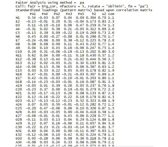
Figure 5.8: Section of the output

When we do this, the majority of the output is a DataFrame with 240 rows labeled Standardized loadings. Each of the rows of this data frame corresponds to a column of our original data frame, such as N1. Remember that these are the questions on the personality profile test that is the source of our data. The first five columns of this data frame are labeled PA1 through PA5. These correspond to each of the five factors we are looking for. The number for a particular personality question and a particular factor is called a loading. So, for example, we have the entry 0.54 in our data frame, corresponding to personality question N1, and factor PA1. We say that question N1 has loading 0.54 on factor PA1.

`We can interpret loadings as contributors to an overall score. To get the final score, you can multiply each particular loading by the survey respondent's answers to each question, and sum up the results. In equation form, we can write this as follows:

Respondent 1's Factor 1 score =

(Factor 1 loading on Question 1) * (Respondent 1's answer to question 1) +

(Factor 1 loading on Question 2) * (Respondent 1's answer to question 2) +

....

(Factor 1 loading on Question 240) * (Respondent 1's answer to question 240)

So, if a factor 1 loading for a particular question is high, then the respondent's answer to that question will have a large contribution to the total factor 1 score. If a loading is low, then the answer to that question doesn't contribute as much to the factor 1 score, or in other words it doesn't matter as much for factor 1. This means that each loading is a measurement of how much each particular question matters in the measurement of a factor.

Each factor has 240 total loadings – one for each question in the personality survey. If you look at the loading matrix, you can see that many questions have a large loading on one factor, and small loadings (close to zero) on all other factors. Researchers frequently attempt to hypothesize an interpretation for each factor based on which questions have the highest loadings for each factor.

In our case, we can see that the first factor, called PA1, has a high loading (0.54) for the first question (labeled N1). It also has a relatively high loading (0.45) for the sixth question (N6), and a high loading (0.62) for the eleventh question (N11). It is easy to see a pattern here – the questions labeled N tend to have a high loading for this first factor. It turns out that these N questions on the original test were all meant to measure something psychologists call "neuroticism." Neuroticism is a fundamental personality trait that leads people to have strong negative reactions to difficulties, among other things. The N questions in the survey are all different, but each is intended to measure this personality trait. What we have found in our factor analysis is that this first factor tends to have high loadings for these neuroticism questions – so we would be justified in calling this factor a "neuroticism factor."

We can see similar patterns in the other loadings:

• Factor 2 seems to have high loadings for "A" questions, which measure agreeableness.
• Factor 3 seems to have high loadings for "E" questions, which measure extroversion.
• Factor 4 seems to have high loadings for "C" questions, which measure conscientiousness.
• Factor 5 seems to have high loadings for "O" questions, which measure openness.

These labels correspond to the "Big 5" theory of personality, which states that these five personality traits are the most important and most fundamental aspects of a person's personality. In this case, our five-factor analysis has yielded patterns of factor loadings that match the pre-existing labels in our dataset. However, we do not need labeled questions in order to learn from factor analysis. If we had obtained data with unlabeled questions, we could still run factor analysis, and still find patterns in the loadings of particular questions with particular factors. After finding those patterns, we would have to look closely at the questions that had high loadings on the same factors, and try to find what those questions have in common.

Linear Algebra behind Factor Analysis

Factor analysis is a powerful and flexible method that can be used in a variety of ways. In the following exercise, we will change some of the details of the factor analysis commands we have used in order to get a better sense of how factor analysis works.

Please note: the following exercise builds on the previous factor analysis code. You will have to run the previously highlighted code, especially big_cor <- cor(big5), in order to successfully run the code in the following exercise.

Exercise 36: More Exploration with Factor Analysis

In this exercise, we will explore factor analysis in detail:

1. We can change several of the arguments in our fa function to obtain a different result. Remember that last time we ran the following code to create our solution:

   solution <- fa(r = big_cor, nfactors = 5, rotate = "oblimin", fm = "pa")

   This time, we can change some of the parameters of the fa function, as follows:

   solution <- fa(r = big_cor, nfactors = 3, rotate = "varimax", fm = "minres")

   In this case, we have changed the rotation method to varimax and the factoring method to minres. These are changes to the behind-the-scenes methods used by the function. Most importantly for us, we have changed the number of factors (nfactors) to 3 rather than 5. Examine the factor loadings in this model:

   print(solution)

   The output is as follows:

   

   Figure 5.9: Section of the output

   You can try to find patterns in these loadings as well. If you find that there is a striking pattern of loadings for three or four or some other number of loadings, you may even have a new theory of personality psychology on your hands.

2. Determine the number of factors to use in factor analysis. A natural question to ask at this point is: how should we go about choosing the number of factors we look for? The simplest answer is that we can use another command in R's psych package, called fa.parallel. We can run this command with our data as follows:

   parallel <- fa.parallel(big5, fm = 'minres', fa = 'fa')

   Again, we have made choices about the behind-the-scenes behavior of the function. You can experiment with different choices for the fm and fa arguments, but you should see substantially similar results each time.

   One of the outputs of the fa.parallel command is the following scree plot:

Figure 5.10: Parallel analysis scree plot

We discussed scree plots in Chapter 4, Dimension Reduction. The y axis, labeled eigen values of principal factors, shows a measurement of how important each factor is in explaining the variance of our model. In most factor analyses, the first several factors have relatively high eigenvalues, and then there is a sharp drop off in eigenvalues and a long plateau. The sharp drop off and long plateau together from an image that looks like an elbow. Common practice in factor analysis is to choose a number of factors that are close to the elbow created by this pattern. Psychologists have collectively chosen five as the number of factors that is commonly used for personality inventories. You can examine this scree plot to see whether you agree that that is the right number to use, and feel free to try factor analysis with different numbers of factors.

The final important outcome of the exercise we have just performed is the scree plot.

You may have noticed that factor analysis seems to have some things in common with principal component analysis. In particular, both rely on scree plots that plot eigenvalues as a way to measure the importance of different vectors.

A full comparison between factor analysis and principal component analysis is beyond the scope of this book. Suffice it to say that they have similar linear algebraic foundations: both are designed to create approximations of covariance matrices, but each accomplishes this in a slightly different way. The factors we have found in factor analysis are analogous to the principal components that we found in principal component analysis. You are encouraged to try both factor analysis and principal component analysis on the same dataset, and to compare the results. The results are usually substantially similar, though not identical. In most real-world applications, either approach can be used – the specific method you use will depend on your own preference and your judgment of which approach best fits the problem at hand.

Activity 13: Performing Factor Analysis

In this activity, we will use factor analysis on a new dataset. You can find the dataset at https://github.com/TrainingByPackt/Applied-Unsupervised-Learning-with-R/tree/master/Lesson05/Activity13.

Note

This dataset is taken from the UCI Machine Learning Repository. You can find the dataset at http://archive.ics.uci.edu/ml/machine-learning-databases/00484/tripadvisor_review.csv. We have downloaded the file and saved it at https://github.com/TrainingByPackt/Applied-Unsupervised-Learning-with-R/tree/master/Lesson05/Activity13/factor.csv.

This dataset was compiled by Renjith, Sreekumar, and Jathavedan and is available on the UCI Machine Learning Repository. This dataset contains information about reviews that individuals wrote of tourist destinations. Each row corresponds to a particular unique user, for a total of 980 users. The columns correspond to categories of tourist sites. For example, the second column records each user's average rating of art galleries, and the third column records each user's average rating of dance clubs. There are 10 total categories of tourist sites. You can find the documentation of what each column records at http://archive.ics.uci.edu/ml/datasets/Travel+Reviews.

Through factor analysis, we will seek to determine the relationships between the user ratings of different categories. For example, it could be that user ratings of juice bars (column 4) and restaurants (column 5) are similar because both are determined by the same latent factor – the user's interest in food. Factor analysis will attempt to find these latent factors that govern the users' ratings. We can follow these steps to conduct our factor analysis:

1. Download the data and read it into R.
2. Load the psych package.
3. Select the subset of the columns that record the user ratings.
4. Create a correlation matrix for the data.
5. Determine the number of factors that should be used.
6. Perform factor analysis using the fa command.
7. Examine and interpret the results of the factor analysis.

   The output should be similar to the following:

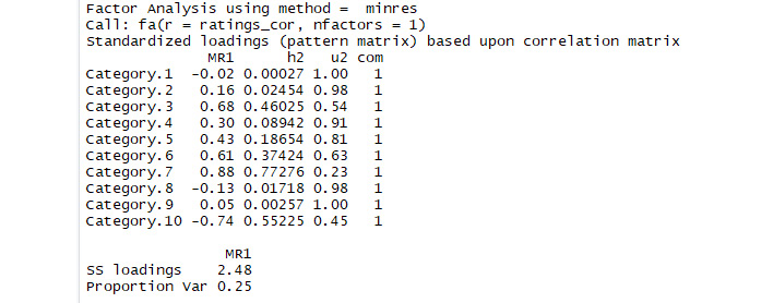
Figure 5.11: Expected outcome of factor analysis

Note

The solution for this activity can be found on page 231.

Summary

In this chapter, we covered topics related to data comparisons. We started by discussing the idea of a data fingerprint. In order to illustrate a data fingerprint, we introduced a hash function that can take any string and convert it to a number in a fixed range. This kind of hash function is useful because it enables us to ensure that data has the right identity – just like a fingerprint in real life. After introducing hash functions, we talked about the need for data signatures. A data signature or analytic signature is useful because it enables us to see whether two datasets are approximate matches – fingerprints require exact matches. We illustrated the use of analytic signatures with image data. We concluded the chapter by covering latent variable models. The latent variable model we discussed was factor analysis. We discussed an application of factor analysis that uses psychological survey data to determine differences between people's personalities. In the next chapter, we will discuss anomaly detection, which will enable us to find observations that do not fit with the rest of a dataset.