
4
Exploration of High-level Synthesis Technique
High-level synthesis (HLS) is a promising technique to increase FPGA development productivity. It allows users to reap the benefits of hardware implementation directly from the software source code specified by C-like languages. This chapter first explores the synthesis process of Vivado_HLS, one of the leading HLS tools. Then, we implement a novel high-convergence-ration Kubelka–Munk genetic algorithm (HCR-KMGA) in the context of a multispectral skin lesion assessment in order to evaluate the technique.
4.1. Introduction of HLS technique
HLS is also called C synthesis or electronic system level synthesis. It allows the synthesis of the desired algorithm specified using the HLS-available C language into RTL and performs the RTL ports connection for the top behavior with specific timing protocol depending on the function arguments. The motivation of this technique is to enable hardware designers to efficiently build and verify their targeted hardware implementations by giving them better control over the optimization of their design architecture and allowing them to describe the design in a higher abstract level.
Despite a series of failures of the commercialization of HLS systems (since 1990s), the innovative and high-quality HLS solutions are always strongly required due to the wide spread of embedded processors and the increasingly fierce market competitions among the electronics manufacturers. Cong et al. [CON 11] summed up the motivations of HLS from the following five aspects:
- – wide spread of embedded processors in system-on-chips (SoCs);
- – huge requirement of higher level of abstraction from the huge silicon capacity;
- – benefits of behavioral IP reuse for design productivity;
- – verification drives the acceptance of high-level specification;
- – trend toward extensive use of accelerators and heterogeneous SoCs.

Figure 4.1. Comparison of RTL- and HLS-based design flows by using Gasjki-Kuhn’s Y-chart: full lines indicate the automated cycles, while dotted lines the manual cycles
HLS is an effective method to reduce the R&D time by automating the C-to-RTL synthesis process. Figure 4.1 compares the conventional RTL with the HLS-based design flows by using Gasjki-Kuhn’s Y-chart [MEE 12]. We can see that the philosophy of this method is to provide an error-free path from abstract specifications to RTL. Its benefits include:
- – reducing the design and verification efforts and helping for investing R&D resources where it really matters. When working at a high level of abstraction, a lot less detail is needed for the description, i.e. hierarchy, processes, clocks or technology [LIA 12]. This makes the description much easier to write and the design teams can therefore focus only on the desired behavior;
- – facilitating behavioral intellectual property reuse and retargeting [CON 11]. In addition to R&D productivity improvement, behavioral synthesis has the added value of allowing efficient reuse of behavioral IPs. Meanwhile, compared with RTL IPs that have fixed microarchitecture and interface protocols, behavioral IPs can be retargeted to different implementation technologies or system requirements;
- – adding to the maintainability and facilitating the updating of the production. Huge silicon capacity may require a large code density for behavior description, which is impossible to be easily handled by human designers for product maintenance or updating. Higher levels of abstraction are one of the most effective methods to reduce the code density [WAK 05].
Xilinx [XIL 13b] reports that its HLS-incorporated product, Vivado_HLS, can accelerate design cycles by around 30% with significant performance benefits related to the conventional methods (see Figure 4.2). Meanwhile, the case of Wakabayashi [WAK 05] shows that a 1M-gate design usually requires about 300 K lines of RTL code, which cannot be easily handled manually, while the code density can be easily reduced by 7–10x when moved to high-level specification in C-like languages, resulting in a much reduced design complexity. Likewise Villarreal et al. [VIL 10] present a riverside optimizing compiler for configurable circuits that achieves an average improvement of 15% in terms of the metrics of lines of code and programming time over handwritten VHDL in evaluation experiments.

Figure 4.2. Design time versus application performance with Vivado_HLS compiler
HLS design flows have significant values. The electronic manufacturers constantly strive to improve their productivity by raising the abstraction level and easing the design process for their engineers due to the increasingly furious market competition worldwide. After an effort of over 20 years, many high-quality HLS tools have been made available for practical applications [MEE 12, PRO 14, RUP 11], i.e. Vivado_HLS of Xilinx [XIL 12b] and Catapult C Synthesis Work Flow [WAN 10]. According to the studies of Meeus et al. [MEE 12], there are five commonly used HLS tools, including Vivado_HLS (Auto Pilot) [ZHA 08], CatapultC [WAN 10], C-to-Silicon [CAD 11], Cyber Workbench [WAK 05] and Synphony C [SYN 10]. Table 4.1 compares their characteristics by using the Sobel edge detection algorithm from eight aspects. Evaluation results are represented by using five levels, --, -, +-, + and ++ from low to high, respectively. The abstraction level evaluates the ability of the tools in terms of timing control. Data types refer to the capability for data format support, such as floating or fixed-point data. Exploration is the design space exploration ability of the tool. Verification evaluates whether the tool can help to generate easy-to-use test benches quickly. RTL quality is estimated by the amount of the hardware consumption of the generated RTL. Documentation is used to evaluate whether the tool is easy to learn or if its documentation is extensive or not. Ease of implementation indicates whether the original source code could be used with fewer modifications or needs to be rewrite completely.
Table 4.1. Characteristic evaluation of five HLS tools
| Auto Pilon Vivado_HLS | Catapult C | C-to-silicon | Cyber WorkBench | Synphony C | |
|---|---|---|---|---|---|
| Source | C/C++ System C | C/C++ System C | C, TLM System C | C, BDL System C | C/C++ |
| Abstraction level | ++ | ++ | + | ++ | ++ |
| Data type | + | + | + | + | + |
| Design exploration | ++ | ++ | - | ++ | +- |
| Verification | ++ | ++ | + | + | ++ |
| RTL quality | ++ | + | +- | ++ | +- |
| Documentation | ++ | ++ | + | +- | + |
| Learning curve | ++ | ++ | -- | + | + |
| Ease of implementation | ++ | ++ | + | + | ++ |
We find that Vivado_HLS has a near perfect performance related to the others. It can benefit the desired design suite in the following aspects:
- – scheduling untimed code (operations) without any restrictions;
- – handling floating-point variables by mapping them onto fixed points: this facilitates the designs of high accuracy applications;
- – providing extensive and intuitive exploration options: with Vivado_HLS, users can discover new solution alternatives by reconfiguring the optimization directives instead of modifying the source code;
- – ability to estimate the running cost of the design: this can facilitate the evaluation of the design candidates and making the final decision;
- – generating high-quality RTL implementations: designers always strive for better design performances within their powers. According to the measuring of Meeus et al. [MEE 12], Vivado_HLS could save up to and more than 95% of hardware resources related to the other 11 HLS tools;
- – easy to be learned even for those who are less knowledgable about FPGAs: this tool can be quickly mastered by C users and requires less hardware knowledge. Furthermore, its documentation is extensive and easy to understand.
4.2. Vivado_HLS process presentation
Vivado_HLS can synthesize the desired algorithm specified using the HLS-available C language into RTL and performs the RTL ports for the top behavior with specific timing protocol depending on the function arguments. Generally, its overall process consists of control and datapath extraction, scheduling and binding, data type processing, optimizations and design constraints. This section discusses the two most important cycles of synthesis process of HLS: control and datapath extraction and scheduling and binding, which may offer most benefits of performance optimization.
4.2.1. Control and datapath extraction
C is a structured programming language that consists of sequential, selectional and repetitional statements, so Vivado_HLS begins the synthesis process with the control and datapath extraction including control behavior extraction, operations extraction and control and datapath creation.

Figure 4.3. HLS control and datapath extraction example: a) input C code source, b) control extraction, c) operation extraction and d) generated control and datapath behavior. For a color version of the figure, see www.iste.co.uk/li/image.zip
First of all, Vivado_HLS analyzes the control logic of the source code to extract its control behavior as a finite-state machine (FSM). For example, the program shown in Figure 4.3(a) is cut into two blocks S1 and S3 by the loop S2. The content of S1 consists of variable declarations and a multiplication operation, S2 is a loop whose body is an If statement and S3 contains only an assignment statement. We assume that all the state transitions can finish their jobs (operations) in a single cycle. Hence, the control behavior FSM for this example should be as shown in Figure 4.3(b).
Next, all the operations in the source code are extracted. Figure 4.3(c) lists all the operations extracted from (a) and classifies them according to the states by the colors of red, green and blue. Since the operation extraction does not take into account register assignments, S1 has only three operations including reading the elements to calculate from array A and B and finding their product. Relatively, the treatment of S2 is more complicated because it does not only have to finish the operations required by the algorithm but also needs some extra operations due to the control logic. Moreover, although each iteration follows only one of the branches in the if-else statement, both of them need to be implemented. Hence, the extracted operations of S2 include a <= and a + for the loop, a == for if-else and three + and a - for the algorithm. S3 assigns the final result stored in temp to the argument dout, so it has only a writing operation. Finally, the extracted operations are assigned to the control behavior FSM and perform the control and datapath behavior shown in Figure 4.3(d).
4.2.2. Scheduling and binding
Scheduling and binding is the key aspect of HLS. The scheduling process determines in which cycles the operations occur, while binding determines which hardware resource or core is used. Figure 4.4 shows the scheduling and binding flow. During this process, the extracted control and datapath behavior and multiple constraints from the device technique libraries and user configurations have to be taken into account, such as the clock frequency, clock uncertainty, timing information, area, latency and throughput directives, etc.
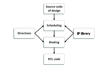
Figure 4.4. HLS scheduling and binding flow

Figure 4.5. Scheduling of the example in Figure 4.3(a). For a color version of the figure, see www.iste.co.uk/li/image.zip
Let us consider Figure 4.3(a) for instance, in which we define the data type as float and two independent interfaces are implemented for Vector A and Vector B. Its default scheduling result with xc7vx1140tg1928-1 of Xilinx is shown in Figure 4.5. In this schematic, a cycle equivalents to a transition from Phase N to Phase N + 1, i.e. RD consumes a cycle because it takes up two phases while ADD does not consume any cycles as it takes only a single phase. Due to the independent interfaces, the RD operations of each vector can be parallelized, so they simultaneously occur in the same phase. According to its control and datapath behavior, S2 is a loop associated with an if-else structure. Generally, the control operations, including ADD, ICMP and SELECT, do not consume cycles, therefore they are usually parallelized with other operations if the sequential relationship allows, i.e. RD A and RD B in Phase 5. Once the comparator in Phase 5 finds that the next iteration will be beyond the loop boundary, it breaks the loop and goes to the next state immediately. In the body of the loop, the two branches of the if statement occur in the same cycles but only one of them is selected via the selector in Phase 11. That is, only one of the two operations is activated in each iteration in the final RTL implementation.
After the scheduling process, the binding process maps the operations to the cores in the technique library. There are generally two binding methods: sharing component and non-sharing component. HLS determines which strategy to use depending on the sequential relationship and technique constraints. Table 4.2 illustrates the operations-cores mapping for the scheduling schematic of Figure 4.5. In this case, FADD and FSUB use the same IP core: faddfsub_32ns_32ns_32_4_full_dsp. Because there are no simultaneously running FADD/FSUB operations in the same cycles, HLS makes them share a single floating-point adder U1. On the other hand, the multiplication operation appears once in the process, therefore only a single multiplier is implemented.
Table 4.2. Operations-cores mapping of the scheduling schematic in Figure 4.5
| Operations | IP Cores | Units |
|---|---|---|
| FADD | faddfsub_32ns_32ns_32_4_full_dsp | U1 |
| FSUB | faddfsub_32ns_32ns_32_4_full_dsp | U1 |
| FMUL | fmul_32ns_32ns_32_3_max_dsp | U2 |
In this section, we can see that the HLS process is highly available to automate the C-to-RTL conversion. Now the question is coming, can the HLS generated RTLs satisfy the industrial level requirements in terms of performance in real-life applications? For this issue, we implement a skin lesion assessment system by using it to evaluate its performance.
4.3. Case of HLS application: FPGA implementation of an improved skin lesion assessment method
The newly introduced ASCLEPIOS [JOL 11] is a promising multispectral imaging system for the assessment of skin lesions (see Figure 4.6). It provides images of skin reflectance at several spectral bands (visible + near infrared spectrum), coupled with software that reconstructs a reflectance cube from the acquired images. The reconstruction is performed by neural network based algorithms. This yields an increase in the spectral resolution without the need for an increase in the number of filters. Reflectance cubes are generated to provide spectral analyses of skin data that may reveal certain spectral properties or attributes not initially obvious in multispectral images.

Figure 4.6. ASCLEPIOS system illustration. For a color version of the figure, see www.iste.co.uk/li/image.zip
Basing on such a system, a KMGA is developed to retrieve the skin parameter maps from the reflectance cube. Using five skin parameter maps such as concentration or epidermis/dermis thickness, this method combines the Kubelka–Munk light-tissue interaction model and genetic algorithm function optimization process to produce a quantitative measure of cutaneous tissue. In this HLS evaluation example, we realize the FPGA implementation of an improved version of the KMGA. During the development, several optimizations are made in order to improve the performances of the final RTL implementation, including optical function rewriting, function optimizer improving and memory optimizing. Obtained experiments demonstrate the high feasibility of low-cost and high-practicability hardware equipment for the clinical system.
4.3.1. KMGA method description
4.3.1.1. Light propagation model in the skin
In order to retrieve the different physical or biological skin properties, several skin models have been developed. The Kubelka–Munk model [KUB 31] is one of the most popular and simplest approaches for computing light transport in a highly scattering medium and has been widely used to model the light-skin interaction. The skin is seen as a 2-layer medium (epidermis and dermis) with five principal parameters that affect the reflectance and transmittance: melanin concentration, epidermis thickness, blood concentration, blood oxygen saturation and dermis thickness. The total reflectance Rtot and transmittance Ttot are expressed as:
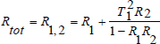
The reflectance Rn and transmittance Tn for a single layer n can be expressed as a function of the thickness of the layer dn, the absorption coefficient μa,n and the scattering coefficient μs, n:
where:
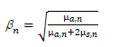
The suffix n equals 1 or 2 for epidermis or dermis. The optical absorption coefficient of epidermis layer μa.epidermis is known as a function of concentration of melanin fmel, the melanin spectral absorption coefficient μa.melanosome and the baseline skin absorption coefficient μa.baseline:
where, with λ corresponding to wavelength parameter,
On the other hand, the dermal absorption coefficient μa.dermis is expressed as follow:
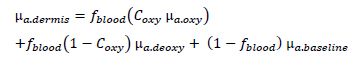
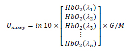
where fblood is the blood concentration in %, Coxy is the oxygen saturation in blood, and μa.oxy are the absorption coefficient of the oxy-hemoglobin and deoxy-hemoglobin in cm-1, respectively. The values of μa.oxy and μa.deoxy with the different wavelengths can be calculated from the Takatani-Graham table using the following equations [JAC 08]:
where HbO2 and Hb are the oxy-hemoglobin and deoxy-hemoglobin content in cm-1/M, G is the hemoglobin’s weight in gram per liter and M is the gram molecular weight of hemoglobin. We selected 150 g/L and 64,500 g/mol as G and M [TAK 79]].
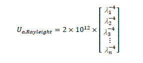
The scattering coefficients of both layers μs,epidermis and μs,dermis are the sum of the Mie scattering coefficient μs,Mie and the Rayleigh coefficient μs,Raylight:
where
4.3.1.2. Function optimizer for skin optical properties retrieval
According to previous equations, it is possible to express R(λ), the total reflectance of the incident light with a certain wavelength, as a function of the skin parameters:
where Depi and Ddermis are the thickness of the epidermis layer and the dermis layer.
The reflectance values are measured with an acquisition system. After a preprocessing step, we can obtain a reflectance cube with two spatial dimensions and one spectral dimension. This cube can be seen as an image where each pixel is described by a vector, representing the reflectance spectrum of the skin as a function of the wavelength (see Figure 4.7). From this measure, the objective is to find the five skin parameters for each pixel that are the most suitable for this measured reflectance spectrum. It is obvious that the KM model is a nonlinear function with five arguments. Several studies have been done about how to solve the similar complex nonlinear function, and the findings of Viator et al. [VIA 05] and Choi [CHO 10] have proved that genetic algorithms (GA) are an effective approach.

Figure 4.7. Reflectance spectrums Sreflectance at a single pixel formed from the reflectance measured: blue and red represent the pixel’s position and green represents the different wavelength values. For a color version of the figure, see www.iste.co.uk/li/image.zip
In KMGA, a candidate solution (called individual) is composed of the reflectance spectrum, skin parameters (fmel, Depi, fblood, Coxy, Ddermis), the spectrum generated by these parameters using equation [4.16] and a fitness value as shown in Figure 4.8. This last one depends on the similarity between the spectrum generated by the parameters and the measured spectrum. It can be expressed by a metric scale such as root mean squared error (RMSE). The set of individuals is called a population.

Figure 4.8. Population data structure: the skin parameters are fmel, Depi, fblood, Coxy and Ddermis. For a color version of the figure, see www.iste.co.uk/li/image.zip
Figure 4.9 illustrates the overall implementation of GA for the KM inversion. First, NP individuals are randomly generated within the range shown in Table 4.3 to form an initial population. Then, in an iterative framework, population evolves by techniques inspired by natural evolution. The evolution of the population is composed of three steps: best individual selection, crossover-mutation and random selection. During the selection process, only the best individuals are kept for the next iteration. Then, the crossover process selects multiple couples of individuals (parents) from the population and one crossover parameter from the five skin parameters to create two new individuals (offspring) by swapping the parents’ selected parameter values. Finally, the mutation process randomly generates some new skin parameter values to replace certain individuals’ old ones. The aim of mutation is to keep exploring the search space and avoid being trapped into a local minimum. These processes are repeated until a predefined number of iterations. Finally, the best candidate is selected.
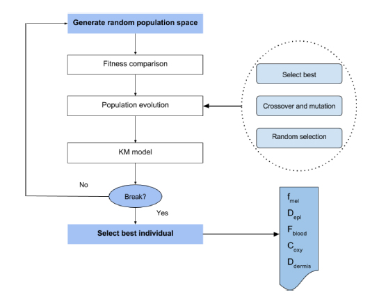
Figure 4.9. Overall genetic algorithm procedure for KM model inversion
Table 4.3. Size of search spaces for skin parameters (see [JOL 13])
| Skin parameter | Symbol | Range |
|---|---|---|
| Melanin concentration | fmel | 1.3-43% |
| Epidermis thickness | Depi | 0.01-0.15 mm |
| Volume blood fraction | fblood | 0.2-7% |
| Oxygen saturation | Coxy | 25-90% |
| Dermis thickness | Dderm | 0.6-3 mm |
4.3.2. KMGA method optimization
KMGA could effectively retrieve the skin parameter maps via a selection process; however, this task is very time consuming even for a powerful processor. Thus, we study a novel HCR-KMGA version in this section. Comparing with its prototype implemented by Jolivot [JOL 11], this implementation can make more acceleration gains according to the following four approaches:
- – HCR-KMGA respecifies the KM function in order to reduce the redundant operations down to a minimum;
- – a prediction function optimization algorithm (PFOA) is designed to accelerate the convergence of the function optimization process;
- – HCR-KMGA individuals’ parameters are optimized depending on the data dependency; some unnecessary data are removed in order to save memory space;
- – multiple different termination conditions are performed in HCR-KMGA in order to avoid the redundant iterations.
4.3.2.1. Function reformulation for computation complexity reduction
According to Figure 4.9, the KMGA method consists mainly of population initialization, population generation and population evolution. Experimental results show that the population initialization and generation takes up to 96% of the total execution time, in which population evolution takes 3% and other operations only 1%. KM is the key technique used during the time-consuming process of population initialization and generation. Thus, in order to speed up the KMGA method, we definitely have to improve its efficiency.
The KM function, the set of equations [4.3]–[4.6], shows that the original model is complex and most parts of its instructions are costly and redundant. For example, the exp(Kndn) term appears four times in equation [4.3]. These redundant instructions are insignificant and costly. It is possible to avoid them by arithmetical reduction. Thus, we reform the KM model:
where FR and FT are optimized KM model functions. These symbols are expressed by:
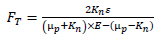
where
The above rewritten KM functions are simple and effective at keeping the processors’ obligations down to a minimum because reading the calculated data from a local register, instead of repeating the computations, can provide a great gain in executive time. Here, exp() is the most costly function, therefore we cut its repetitions down to only once per iteration by combining like terms and defining two interim storing registers E and ε. The other instructions are also reduced more or less by similar approaches. Table 4.4 compares the number of necessary instructions between the initial prototype and our implementation: the optimized function requires fewer instructions than before.
Table 4.4. Necessary instruction number comparison between original and optimized KM functions
| Model | Addition/subtraction | Multiplication/division | Exponentiation |
|---|---|---|---|
| Original KM | 13 | 17 | 13 |
| Optimized KM | 8 | 9 | 3 |
On the other hand, section 4.3.1 presents that the optical absorption and scattering coefficients of epidermal and dermal layers are ultimately functions of wavelength and skin parameters. We can reformulate equations [4.7], [4.10] and [4.13] by using vector equations:

where
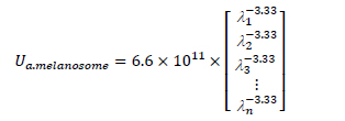
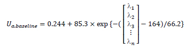


In equations [4.23]–[4.31], Ua.melanosome, Ua.baseline, Ua.oxy Ua.deoxy, Ua.epidermis and Ua.dermis are six coefficient vectors with different wavelengths. They are fixed from 450 to 780 nm with a step of 10 nm. These vectors can be precalculated and stored in the memory. Thus, instead of calculating the values wanted at each iteration, the processor is able to read them directly from the memory. This approach avoids all the repeated computations due to equations [4.8], [4.9] and [4.11]–[4.15] in the routine.
4.3.2.2. Convergence acceleration of function optimizer
It is obvious that equation [4.16] is a complex nonlinear function with five arguments, which is impossible to inverse by mathematical methods. KMGA optimizes this function according to a standard genetic algorithm. This optimization process is a search heuristic that mimics the process of natural selection. It generates solutions to optimization problems using techniques inspired by natural evolution, such as inheritance, mutation, selection and crossover. It has also proved effective in the application of bioinformatics, phylogenetics, computational science, engineering, economics, chemistry, manufacturing, mathematics, physics and pharma-cosmetics, etc. However, the evolution process of a pure natural-simulated genetic algorithm is time consuming, and can easily get trapped into local optima. This is because GA always generate the new populations in a random way first and then selects the best individual according to the fitness function, which enormously reduces the chance to find a better individual in the next iteration that results in a very low convergence rate. Thus, within HCR-KMGA, we perform a PFOA optimization process, which can raise the convergence rate by predicting the possible evolution directions.

Figure 4.10. Overall architecture of the prediction function optimization algorithm (PFOA)
Figure 4.10 illustrates the overall architecture of PFOA. Like the conventional GA, the system first randomly initializes the population. However, in the evolution process, only the best individual selection process is kept, while crossover-mutation and random selection are replaced by predictive evolution and random evolution. After each iteration, the best individuals are directly copied from the last generation into the next one for the purpose of fast convergence. Meanwhile, some of the individuals move depending on a prediction strategy, which can further raise the convergence rate of population evolution by a considerable amount. Finally, the rest of the individuals are re-performed randomly in order to reduce the possibility of falling down to the local optima.
Depending on different fitness functions, designers can customize different prediction strategies. In our case, an individual has five skin tissue parameters and the size of population consists of a few hundred individuals. In each iteration, several new genes are generated via the crossover-mutation process. However, with the floating-point number, which is one of the most frequently used data formats in computer science, KMGA has more than 6E27 candidates (this value is estimated according to the range of the five skin parameters shown in Table 4.3 and the precision of the floating-point numbers), which may result in a long running time and a very low convergence rate.

Figure 4.11. Search space prediction of PFOA: xn and fn are the parameter and fitness value of the nth iteration’s best individual, (x0’, f0’) is the local optima and (x0, f0) is the global optima of the optimization function
For the purpose of accelerating the convergence speed of the algorithm, a prediction strategy that can reduce each iteration’s search space by predicting the evolution direction is performed as shown in the right of Figure 4.10. First, the best individuals of the last two generations are compared and, depending on the comparison result, the algorithm takes different steps to adjust the search space. We base the prediction strategy on the assumption that higher parameter values had better fitness while xn-1 > xn-2 and lower parameter values had better fitness while xn-1 > xn-2 where xn refers to the parameter value of the best individual of the nth generation. As shown in Figures 4.11(a) and (b), PFOA locks the search space U onto the scope of x > xn-1 with xn-1 > xn-2, while the scope of x < xn-1 with xn-1 < xn-2. Meanwhile, we note that this method is effective only for the situations in which the present best individual is far enough away from the optima. Once it is closer to the optima, a much smaller search space may be required to enable the algorithm to find a better individual with as few iterations as possible. This situation is abstracted as xn-1 = xn-2 and f(xn-1) = f(xn-2) in PFOA. It means that no better individuals are found in the last two iterations. Therefore, the search space of the nth iteration will be locked within the scope around xn-1 in order to enhance the chance of evolution (see Figure 4.11(c)).
Since the optimization function is unknown, it is impossible to always correctly predict the position of the global optima. However, this mistake can be quickly corrected in the following iterations. For example, the predicting scope does not include the optima in Figure 4.11(b) and within this scope no better individual can be found. However, this makes the algorithm restrict its search space around xn-1 in the following iterations, within which a new best individual can be easily found in the right of xn-1.
The KM model has five parameters to be figured out. Considering that these parameters have different effects on the final fitness, their analyses must be independent from each other. Thus, HCR-KMGA applies PFOA to all of them respectively. That is, after the fitness comparison, the search space of each parameter is defined independently via the proposed prediction strategy.
It should also be noted that sometimes this method may also lead the evolution down to local optima. Thus, after prediction evolution, some random individuals are performed in order to avoid this outcome. Unlike GA, PFOA completely regenerates all the individuals in a random way instead of crossovers or mutations. This method greatly enriches the sample types of genes, so the risk of missing the optima is reduced.
4.3.2.3. Individual information storage optimization
Figure 4.8 shows that the information of an individual consists of fitness value, chemical properties (skin parameters) and optical properties (simulated spectrum). These data need to be saved in the memory of the processing device permanently throughout the whole processing, and therefore the conventional KMGA prototype has to consume a lot of hardware resources to store all the population information, especially for embedded devices. Thus, an approach that can reduce memory consumption is required.
According to the algorithm analysis, it is found that each piece of individual information is not isolated but rather has internal relations with the others. Figure 4.12 displays the relationships among them and it demonstrates that both the simulated optical properties and the fitness value are calculated from the chemical properties. That provides a nice opportunity to compress the data size by removing the data that could be computed immediately and keeping only the necessaries.
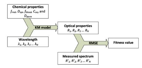
Figure 4.12. Relationships of individual date
The individuals of HCR-KMGA are performed by chemical properties and fitness values, while the information of its simulated optical properties is removed. In the overall algorithm, the simulated spectrum of the skin lesion zone is used only once in order to compute the fitness values for the best individual selection at the beginning of each iteration (see Figure 4.10) and it is therefore unnecessary to allocate a certain memory to store them. Meanwhile, a single fitness value takes up only several octets while its computing has to call the KM models, which has a very long running time. Nevertheless, this data is required not only in the best individual selection process but also in the prediction evolution process. Thus, this number is stored as part of the individual information in HCR-KMGA in order to accelerate the design by reducing the operations number. The data size comparison between KMGA’s and HCR-KMGA’s individual could be expressed as follow:
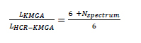
where LKMGA and LHCR-KMGA are the total data length of the two algorithms’ individuals and Nspectrum is the number of bands of the spectral image. Obviously, HCR-KMGA consumes much less memory space than KMGA and its total length is permanently six times the defined number length. That is, the algorithm will not take any more hardware resources for the population information storage even for spectral images with high bands numbers.
4.3.2.4. Iteration termination conditions
The evolution process of a GA is terminated after a number of iterations according to the termination conditions customized by designers. A main issue that always affects the selection of termination conditions is that defining a condition which is easy to reach consumes fewer hardware resources but may reduce the accuracy performance of designs, while a hard condition may lead to extensive computational time and the algorithm can even be trapped in an infinite loop.
KMGA terminates the evolution process by defining an iteration number which corresponds to the convergence of the population. That is, the evolution stops when the iterations number reaches the default value. This approach could provide an acceptable average fitness value for the processing of a standard skin lesion multi-spectral image. However, the computation of GA is full of all kinds of possibilities, so such a simple termination condition may lead to redundant iterations or unpredictable results. For example, the evolution process will not be terminated until it reaches the default iterations number even if the global optima has been found, or alternatively the evolution process may have been terminated before the fitness reaches the required level. Thus, instead of forcing the algorithm to end by setting a default iteration limitation, HCR-KMGA combines multiple termination conditions together, including max continuous invalid iteration level θinvalid.iter, fitness level θfitness and total iteration level θtotal.iter.
In our work, an iteration in which a new best individual is found is called a valid iteration, otherwise it is an invalid one. Once a large number of continuous invalid iterations appear, it means that the present best individual is very close to the optima and it will be difficult or time-consuming to find another one for the algorithm. So in order to save the hardware resources, a max continuous invalid iteration level is defined to break the evolution loop while no new best individual is found during θinvalid.iter iterations.
Normally, the goal of evolution is not to exactly figure out the optima. That is, a fitness error could be accepted in each processing. In HCR-KMGA, a fitness level refers to the acceptable fitness error. Once the fitness value of the present best individual is lower than the fitness level, the evolution loop could be broken as well.
Finally, in order to avoid the algorithm getting trapped in an infinite loop, a total iteration level is defined. It should be noted that these three termination conditions simultaneously effect the algorithm, so no matter which one is reached, the iterations will be ended. This method can save as many hardware resources as possible, and meet the accuracy requirements of the design as well.
4.3.3. HCR-KMGA implementation onto FPGA using HLS technique
As one of the most popular computation platforms, FPGAs have been used in a wide variety of real-time image processing applications. Depending on the proposed HCR-KMGA, a FPGA-based embedded skin lesion assessment system is realized in this section.
4.3.3.1. Development flow
Figure 4.13 illustrates the HLS-based development process used for the implementation. After a careful algorithm analysis, we first realize a synthesizable KMGA prototype in C language. Next, the prototype is optimized by using the approaches discussed in section 4.3.2 and simulated through a common C compiler, i.e. Intel C++ Compiler (ICC) [INT 08]. Third, the functionally verified source code is imported into the HLS tool for C-to-RTL synthesis. During this process, the synthesis directives are carefully configured in order to effectively use the hardware resources of the target device. Finally, the IP block of HCR-KMGA is automatically performed for top behavior.
4.3.3.2. Functional block implementation onto FPGA device
The over-all architecture of HCR-KMGA is shown in Figure 4.14. Its initial population is generated according to the skin parameters’ value range presented in Table 4.3. As mentioned in section 4.3.2, we replace the calculation of μa.mel, μa.baseline, μa.oxy, μa.deoxy and μs.epidermis with different wavelengths by a coefficient table pre-calculated using the Takatani–Graham table [TAK 79]. As there is no golden rule to define the values of evolution process parameters, we base HCR-KMGA’s parameters configuration on the results of intensive tests. In the fitness computation, RMSE is applied as the metric scale to compare the candidates’ simulated optical properties with the reference spectrum.
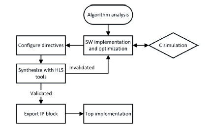
Figure 4.13. Development process for the HCR-KMGA’s FPGA implementation
PFOA’s evolution process consists of best-individual selection, prediction evolution and random evolution processes. Moreover, in order to make the routine synthesizable, the standard C function rand(), which is not supported by the HLS tool due to the use of static variables, is replaced by a linear congruential random number generator coded manually:
where X is the sequence of random values, m (m > 0) is the modulus, a (0 > a > m) is the multiplier, c (0 <= c < m) is the increment and X0(0 <= X0 < m) is the start value (also called seed).
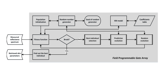
Figure 4.14. Software implementation of HCR-KMGA algorithm for the FPGA device
4.3.3.3. Parameter configuration
As there is no golden rule to define the value of the GA parameters, we perform the configuration through a series of tests. Table 4.5 compares the parameter configurations of KMGA and HCR-KMGA.
Table 4.5. Population parameter configuration for KMGA and HCR-KMGA
| Parameters | KMGA | HCR-KMGA |
|---|---|---|
| Population size | 100 | 100 |
| Best individuals | 10 | 1 |
| Random selection individuals | 30 | - |
| Crossing individuals | 30 pairs | - |
| Mutation individuals | 3 | - |
| Prediction individuals | - | 49 |
| Random individuals | - | 50 |
| Maximum fitness plateau | - | 6 |
| Minimum satisfies fitness level | - | 2E-4 |
| Max generation number | 25 | 80 |
| Spectrum size | 34 | 34 |
Both the crossing and mutation of KMGA were selected from the literature [SYS 89] and take the probability value Pc = 0.6 and Pm = 0.02, respectively. We did not want to select a high mutation probability as it is noticed that the convergence was not smooth and often temporarily increased.
4.3.4. Implementation evaluation experiments
According to the algorithm described in sections 4.3.1 and 4.3.2, we can see that the KMGA and HCR-KMGA are highly parallelizable at the pixel level but the computation of each pixel is much less parallelizable and intensive due to the iteration structure of the evolutionary algorithm and complex KM function. Therefore, besides FPGA, the CPU implementation of KMGA is selected as the reference in order to obtain an unbiased evaluation. In this section, we first introduce the reference CPU implementation and then analyze the performance gains due to the algorithm improvement. Finally, the performances of the proposed FPGA design and the reference implementation are compared.
4.3.4.1. Reference optimizations: parallel computing within GPP
We select the GPP implementations of KMGA and HCR-KMGA as references. Both of them are realized on a Quad-Core CPU Q6600 (Intel CoreTM Quad CPU Q6600 @ 2.40 GHz X 4) with ICC 13.1.1 in 32-bit in the Ubuntu 13.04 system. In order to obtain an unbiased comparison, they are optimized using recent parallel computing technique Pthreads to achieve as many as possible potential performance gains from the target multi-core CPUs.
For the purpose of achieving more effective use of hardware resources in a multiple-core environment, many parallel programming methods have been developed [AYG 09, KYR 11, STR 08]. A series of studies have demonstrated that the parallelization architecture can greatly improve the image processing prototypes’ efficiency [AKG 14, BAR 14, BIS 13, HOS 13, TOL 09]. Pthreads is one of the most popular parallel programming technologies for UNIX-like operation systems. This method allows multiplying the speed of the designs by simultaneously executing multiple threads depending on the available core number of the target processor. Comparing to the other methods, Pthreads’ advantages consist of the rapid thread creation [BAR 17], the shared global memory and the private data zone for each thread, so the Pthreads implementations may gain more potential improvement in the running time and hardware cost performances.
In parallel programming, the first step is usually to find out the independent data flows in the original algorithm. Figure 4.15 illustrates that KMGA method analyses each single pixel’s reflectance spectrum. That is, the algorithm sweeps all over the lesion zone pixel by pixel, and their data flows are independent of each other. This intrinsic nature of KMGA provides a nice parallelization potential.

Figure 4.15. N-threads KMGA architecture using POSIX threads: Sreflectance_n is the reflectance spectrum at (in, jn) in the work area of the nth thread and Ppixel_n is its retrieved skin parameters. For a color version of the figure, see www.iste.co.uk/li/image.zip
Using the Pthreads technology, we designed a single program multidata parallelization as shown in Figure 4.15. Within this architecture, the multispectral image and retrieved skin parameter maps are stored in two allocated shared memory regions in floating-point format. Meanwhile, the original image is divided into N work areas and each of them is distributed to a single thread. Since all the data flows are independent, there are no interactions between two threads. Once the processing of a distributed reflectance spectrum is finished, the thread accesses the shared memory again with a store address in order to write data into the right position and then starts another operation. During the processing, parallel threads need only to traverse their flown data segment.
In addition, given that a multicore superscalar processor is selected as hardware platform, the operations are scheduled according to a multiple instruction multiple data (MIMD) strategy, which allows a superscalar CPU architecture to execute more than one instruction during a clock cycle by simultaneously dispatching multiple instructions to different functional units on the processor such as an arithmetic logic unit, a bit shifter, or a multiplier. For example, the computations of equation [4.23] consist of two independent terms fmel Ua.melanosome and (1-fmel) Ua.baseline. MIMD can therefore accelerate computations by scheduling their instructions in parallel rather than make the algorithm run them one by one via a superscalar CPU architecture. Moreover, Pthreads can be automatically scheduled depending on the cores number in an out-of-order execution way by the compiler, therefore the developers have no need to consider the compatibility between the thread numbers implemented and the core number to make the processor run at full load all the time. This allows an effective use of processors resources and an important acceleration of the desired operations.
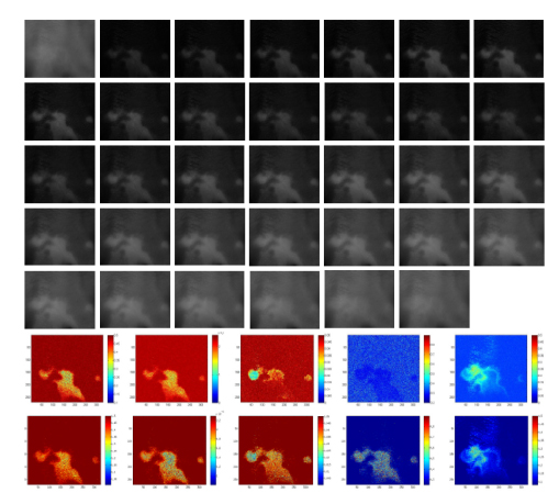
Figure 4.16. Multispectral image measured by ASCLEPIOS from 450 to 780 nm with a step of 10 nm (top), and simulation results of five maps obtained by KMGA (middle) and by HCR-KMGA (bottom). These five maps (from left to right) consist of melanin concentration, epidermis thickness, volume blood fraction, oxygen saturation and dermis thickness. For a color version of the figure, see www.iste.co.uk/li/image.zip
4.3.4.2. Comparison experiments
Figure 4.16 displays the skin parameter maps retrieved by KMGA and HCR-KMGA from a standard multi-spectral image. Obviously, the latter makes less noise from the visual effects and provides a clearer skin lesion zone for diagnostics. According to the test results, we can find that the HCR-KMGA implementations have lower fitness values than the KMGA ones (2.6 × 10⁻⁴ vs. 3.4 × 10⁻⁴; lower is better). Meanwhile, note that the fitness values are almost identical to the FPGA and CPU implementations. This is because the HLS-based SW/HW co-design framework can effectively transplant an algorithm specified in C-like languages onto FPGAs almost without any omissions of functions.
The efficiency performances of all implementations are compared in Table 4.6. Due to the prediction evolution strategy, HCR-KMGA offers an acceleration gain of 2.28× relative to KMGA, while there is a gain of 2.13× for FPGA-HCR-KMGA versus FPGA-KMGA. Nevertheless, the looplevel and instruction-level parallelism enable FPGAs to appear to provide much better hardware performances than CPUs, although they have a lower clock frequency. The speed gains due to the platform are 5.84× and 5.45× for FPGA-KMGA versus KMGA and FPGA-HCR-KMGA versus HCR-KMGA, respectively.
Table 4.6. Implementation acceleration ratio comparison: the clock of CPU and FPGA are, respectively, 2.4 GHz and 50 MHz
| KMGA | HCR-KMGA | FPGA-KMGA | FPGA-HCR KMGA |
|---|---|---|---|
| 1 | 2.28 | 5.84 | 12.432 |
Finally, we compare the hardware resources consummation of the two FPGA implementations in Table 4.7. This comparison indicates that HCR-KMGA consumes much less RAM than KMGA. This is because the data size of the population are well reduced according to the approach presented in section 4.3.2; it therefore need not allocate as much storage space as before. In contrast, HCR-KMGA consumes more than other components; this is because PFOA has a more complex architecture than GA and HLS has to spend more resources for the operation control flow. However, this difference is very tiny; it can almost be ignored in practical applications.
Table 4.7. Used hardware resources estimation of FPGA-KMGA and FPGA-HCR-KMGA implementations on Virtex7-XC7VX1140T of Xilinx
| Components | FPGA-KMGA | FPGA-HCR-KMGA |
|---|---|---|
| BRAM_18K | 192 | 32 |
| DSP 48E | 2352 | 2431 |
| Flip-Flop | 467264 | 493177 |
| LUT | 668784 | 712894 |
4.4. Discussion
This chapter explores the fundamental concepts of HLS technique according to an example of an embedded skin lesion diagnostic application, which combines a complicated skin light propagation model, KM model, and a high running cost function optimizer genetic algorithm. Historically, this case should have required a significant effort cost to be implemented onto FPGAs even for an experienced FPGA engineer due to the large gap between the algorithm complexity and the low abstraction level of register-level languages. However, with the help of HLS, we do not have to suffer of the complexity of the low-level logic control and data flow any more. Nevertheless, since the behavior block is specified in standard C language and synthesized automatically, we can quickly switch the desired compilers (ICC and Vivado_HLS) without manually respecifying the behavior block in RTL after the function verification in the software environment. This allows us to put more attention into algorithm and architecture improvement.
Thanks to the benefits of HLS, we can focus exclusively on the desired behavior description and propose a new HCR-KMGA. A series of complicated optimizations are made on the target design. According to the algorithm evaluation experiments, the new proposed algorithm doubles the convergence speed of the evolution process and achieves a higher accuracy.
In addition, the operation scheduling of the target implementation is optimized by using HLS directives. The final RTL is compared with the multicore implementation optimized through Pthreads. The experiments demonstrate that FPGAs achieve a speedup of around 6× in hardware terms. However, this optimizing process is still painful for software engineers who are not familiar with HLS and FPGAs because RTLs are constrained by hardware resources and the features of the target devices that differ from the GPP. In Chapter 5, we further discuss the HLS-based design flows and propose a code and directive manipulation strategy for efficiency optimizing.