
An old Far Eastern proverb advises that “a picture is worth a thousand words.” The truth of the proverb is fully realized in chemical analysis and medical imaging where not only the numerical values but the shape of the recorded data conveys information. Numerous techniques in medical, physical, and many other experimental sciences depend upon the graphical presentation of data. Clinical and chemical analysis has traditionally used chemically sensitive transducers to generate a millivolt signal in response to changing chemical process values. The small signal was amplified electronically and used with a servomotor to mechanically drive a pen across a paper chart to provide a visual record of the chemical process being monitored. Although both x-y and x vs. time plotting systems are extensively employed in the manufacturing process industries, chemical analysis, and other sciences, the electro-mechanical plotting instruments, much like the typewriter, have been replaced by the PC.
x-y plotting is used extensively in analytical spectroscopies and electrochemical analysis, while x vs. time charting is used for following titrations, in biochemical kinetics, and in both chromatographic and spectroscopic analysis.
DAQFactory is being used for this application because of its powerful graphical recording and display capabilities. A graphical display tutorial is included with the DAQFactory user manual along with a detailed chapter on the DAQFactory graphical display capabilities. Both the tutorial and the user manual should be reviewed before starting this exercise for those researchers using either the free Express or full version of the SCADA software.
In this exercise, several very important concepts and circuit configurations are demonstrated. The 555 timer configured as an astable multivibrator will be used to create square, sawtooth, and nonsymmetrical triangular signal waveforms as a prelude to visually examining the very important concept of pulse width modulation (PWM). Exponential and linear voltage waveforms from capacitor charging and discharging will be demonstrated, and the creation of symmetrical voltage waveform outputs from special ICs will be used for creating graphical data recordings.
In the first timer configuration examined, two resistors and a capacitor will be used to form a “timing network ” on the oscillator chip. The RC component values will be chosen so the timer chip generates waveforms compatible with our recording software. One of the resistance components chosen will be of a variable nature to model a resistance-based chemical or physical transducer. Variation of the transducer resistance with some physical phenomenon, such as the intensity of the light falling on the sensor surface or temperature, will then cause the frequency and wavelength of the timer output signal to vary, and the output variation will be displayed on the PC screen in a graphical format. Signal variation can then be transformed into pulse width variation to form the basis of the extensively used pulse width modulation (PWM) concept.
In the second timer configuration examined, the use of a constant current source to charge the timing capacitor will be demonstrated, and the creation of “sawtooth” and triangular output waveforms will be graphically recorded. The triangular waveform or voltage ramp has an important use in some sensor monitoring and in chemical analysis. A third circuit is assembled to demonstrate a simplified method for creating a dual-slope analog ramp that is used frequently in electrochemical, corrosion, and biophysiology investigations.
A simple x-y recording system constitutes the last portion of the chapter.
Experimental: Linear Graphical Data Recording
Part 1: Hardware and Component Selection – Square Wave Output
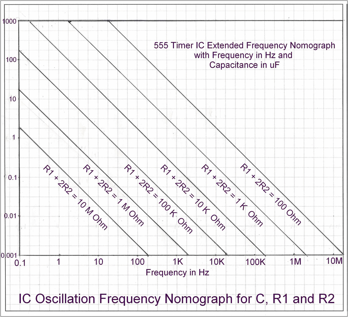
555 Timer Output Frequency for R-C Timing Network Values
In order to keep the output signal from the timer chip in the low frequency range that should be suitable for the DAQFactory graphics, the resistance values should be in the megohm range (million or 106 ohms) and the capacitance value in the 0.1–10 uF (micro or 1/1,000,000 F) range. The graphical data of Figure 9-1 is an approximation, and the actual resistance values chosen for use are somewhat dependent upon the capacitance value selected or available.
An electrolytic capacitor with a value of 1–10 uF should be suitable for this graphics display exercise, but for more accurate work, a higher-quality low-leakage type of capacitor may be required as detailed in the following discussion.
Electronic Components Required
- 1)
555 timer integrated circuit
- 2)
Variable and fixed resistors to sum into the low megohm range preferably with the fixed and variable values being in the same order of magnitude of resistance
- 3)
A suitable “timing” capacitor in the 1–10 uF range, a 0.01 uF bypass capacitor, and a 9 V battery supply
Circuit Schematic
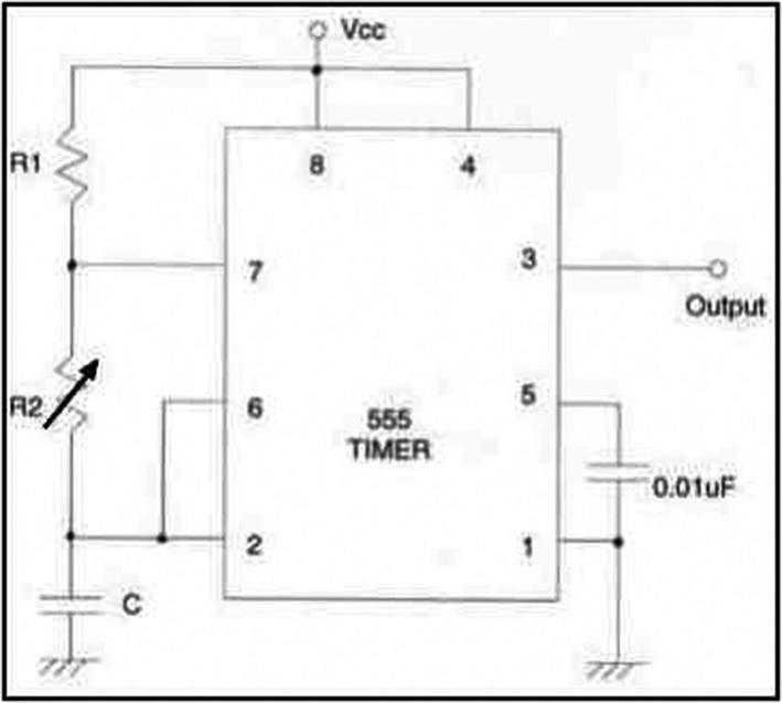
555 Timer Astable Configuration
The preceding circuit shows a single variable resistance between pins 7 and 2. The circuit will work when the variable resistor is in its mid-travel position but will produce erratic results when at the low end of its resistance value. To avoid any problems with circuit malfunctions, place a fixed value resistor in series with the variable unit to limit the lower end value of the second timing network resistance. The author used a 10 kΩ value for a 1.2 MΩ R1 + R2 network sum value.
Software
After having assembled the astable oscillator, connect the output to a differential input channel on the LabJack and configure a channel for receiving the square wave output. The graphical page component can then be created. For long-duration graphical displays, make sure the channel storage capability is large enough to support the length of the desired time display. The number of values in memory is defined by the value in the channel's “History” box. (The default entry is 3600 that can be filled quite quickly when working in experimental time frames of tens of minutes or fractions of hours.)
Page Components Required
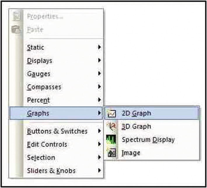
DAQFactory Selection of a 2D Graphical Recorder Screen Display
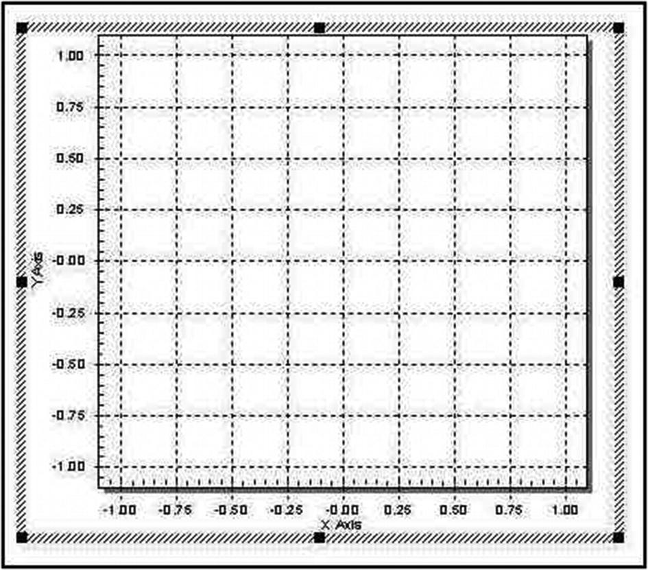
The Default X-Y Graphical Screen Display

Recorder Trace Name Selection
A Help screen at the bottom of the properties window explains all of the data entry boxes and tabs that are found in the graphical screen component.
For the square wave being generated by the 9-volt battery-powered 555 timer oscillator, the voltage range was offset to display values from –1 to 9 volts to more clearly depict the time the waveform is at 0 V.
Part 1: Observations
With a 392 kΩ R1, a 900 kΩ R2, and a 10 kΩ series resistance limiting unit, charging a 22 uF, 25 V electrolytic capacitor from a 9 V battery, a graphical display of four high time cycles in 60 seconds was obtained with a midrange setting on R2.
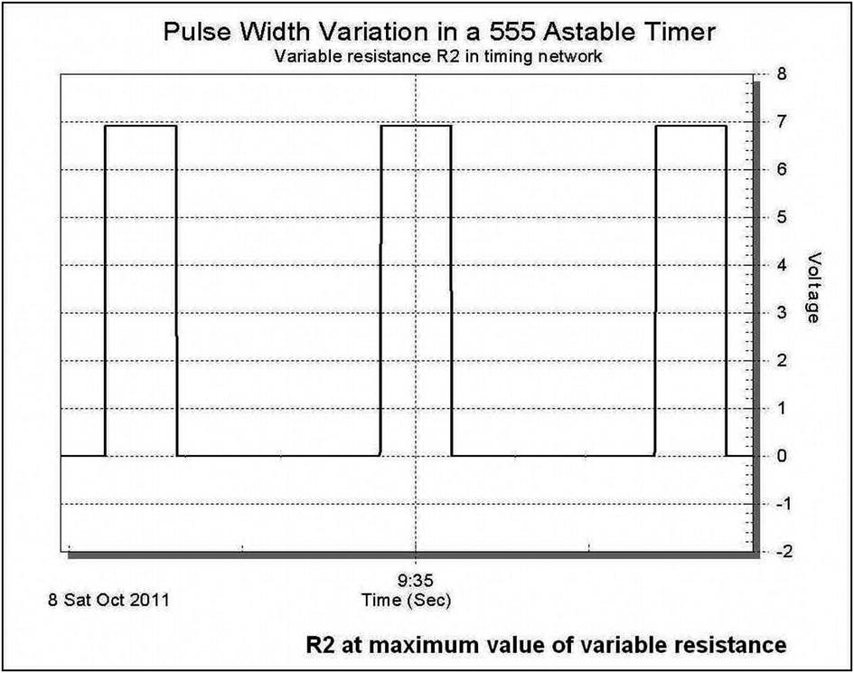
Timer Output at Maximum Resistance
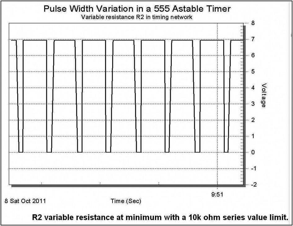
Timer Output at Minimum Resistance

Waveform Without Minimal Resistance
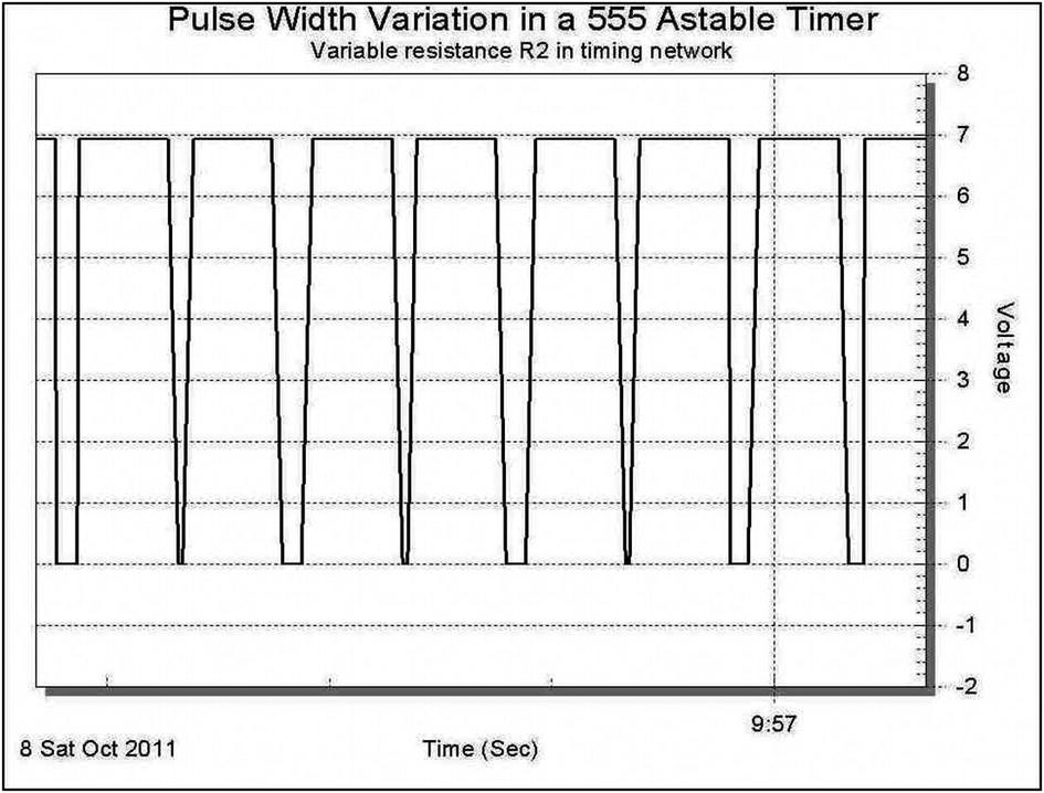
Erratic Output Signal or “Aliasing”
Experimental
Part 2: Hardware and Component Selection – Triangular and “Sawtooth” Outputs
In addition to the creation of a square wave signal with a varying duty cycle, the astable 555 timer can be used to generate a “sawtooth” and asymmetrical triangular wave. Basic electronics teaches that when a capacitor is charged or discharged through a fixed value resistor, an increasing or decreasing exponential voltage value is seen across the terminals of the capacitor. When a capacitor is charged with a constant current source, a linear voltage increase is seen across the capacitor terminals. The linear voltage change forms a triangular waveform that can be used to generate a voltage ramp having several applications in chemical analysis and other experimental work.

A Constant Current Charging Source
Part 2: Observations

Typical 555 Timer “Sawtooth” Output Voltage Waveform

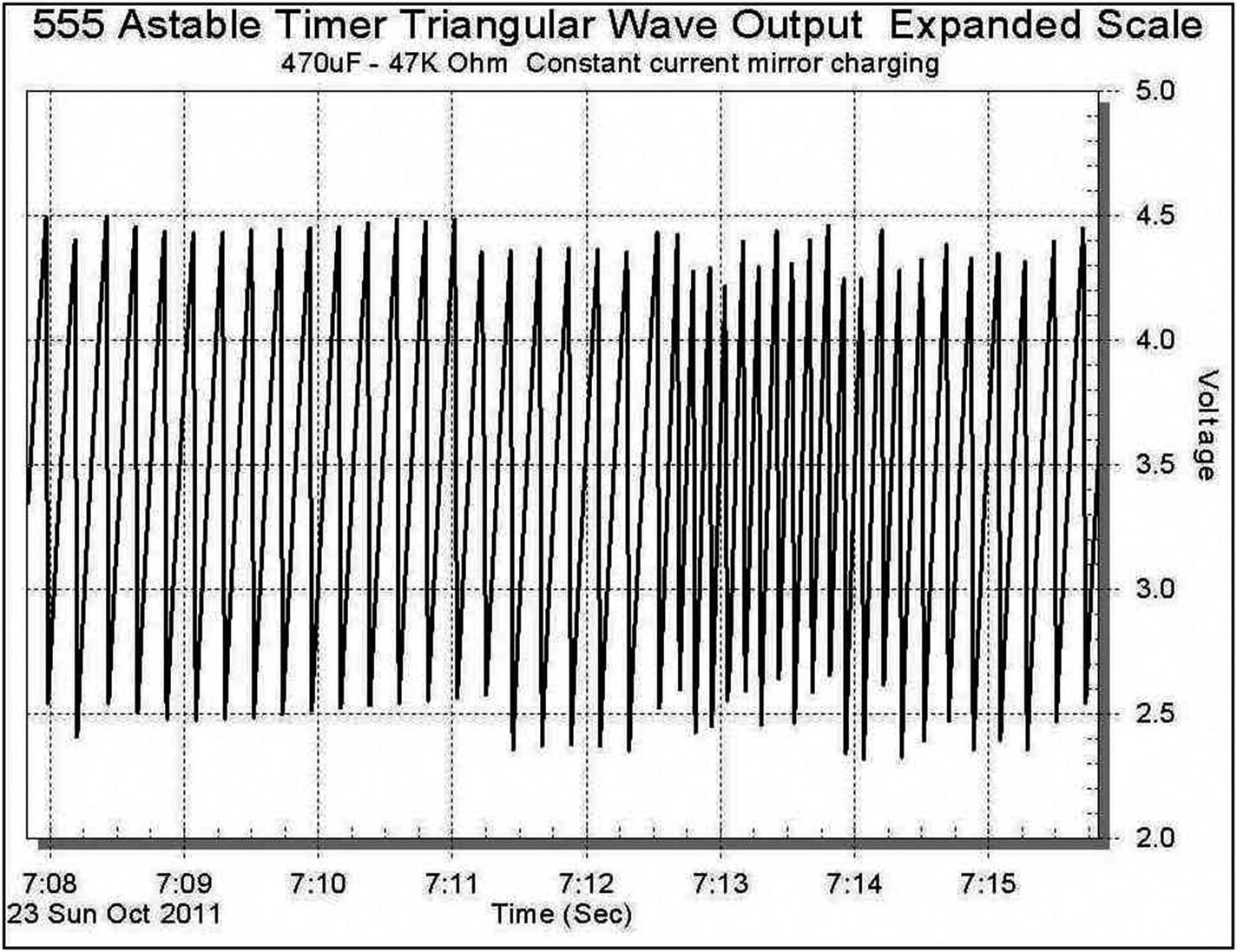
A 555 Timer Triangular Wave Expanded Scale

The Effect of Added Discharge Resistance on the Timer Output Waveform
Simple logic would suggest that to obtain a linear triangular waveform, charging and discharging a capacitor through constant current sources and sinks would achieve the desired result, but a simpler solution can be found by using “function generators” that can produce signals of various shapes and frequencies.
Part 3: Hardware and Component Selection – Dual-Slope Triangular Waveform
Schematic for Function Generator Configuration
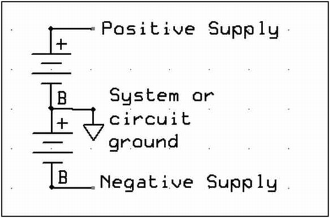
A Dual-Battery Bipolar Power Supply
If the circuit, when properly assembled on a breadboard, fails to operate as expected, consult the manufacturer’s data sheets and the “Discussion” section.
Part 3: Observations

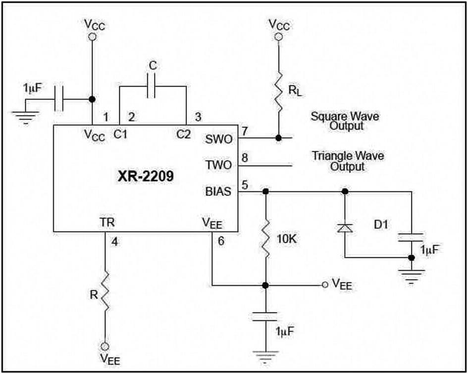
XR-2209 Function Generator Symmetrical Triangular Wave Output
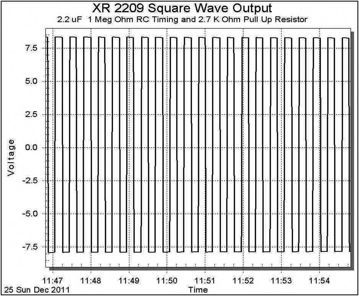
Square Wave Output with Pull-Up Resistor
X-Y Data Recording
As can be seen in Figure 9-4, the default format for the two-dimensional plotting, graphical display screen component is x vs. y. The constant current charging circuit of Figure 9-10 can be used to produce an x-y plotting of the voltage across the capacitor and its square as would be used in measuring the energy developed across the capacitor. E = CV2/2. The constant current circuit can be used for this demonstration exercise because an asymmetrical voltage ramp is created on the capacitor by the constant current charging and the exponential discharging of the component.
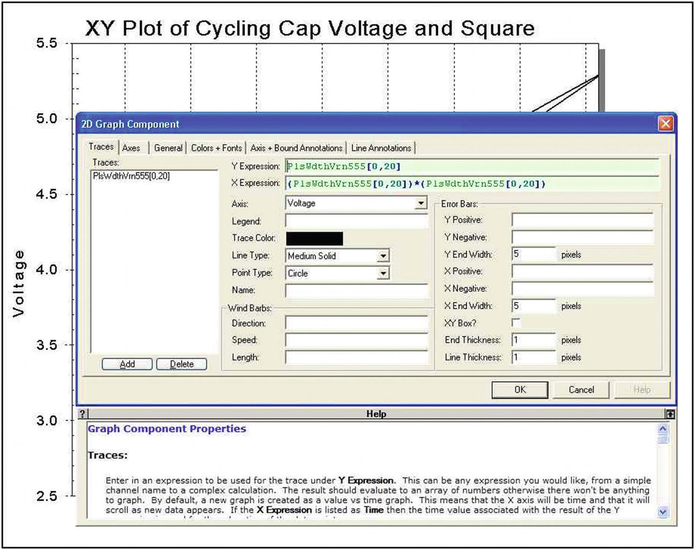
x-y Graph Traces Tab
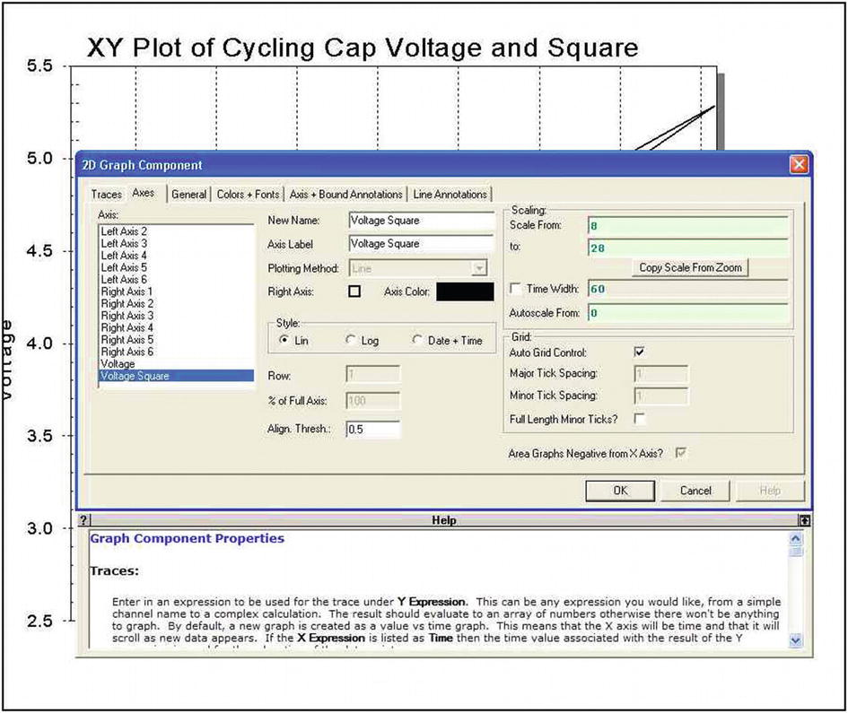
x-y Graph Axes Tab
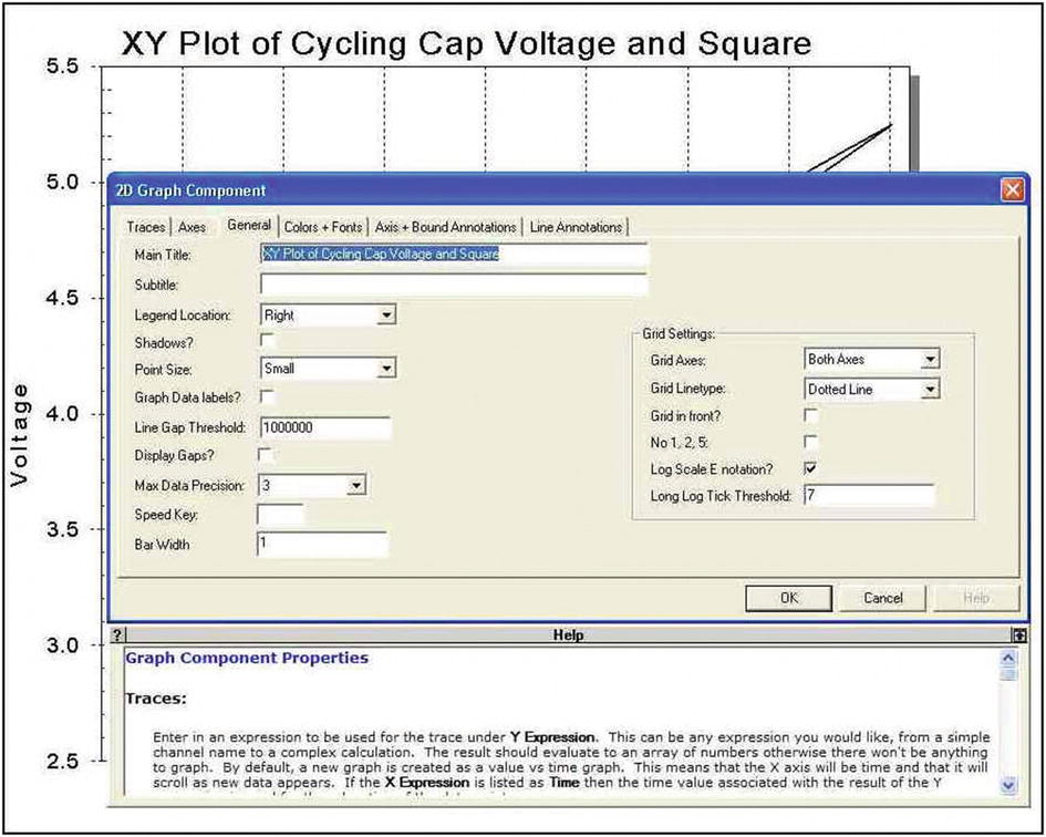
x-y Graph General Tab

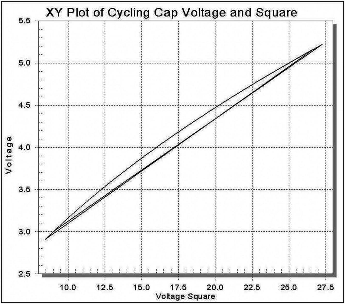
A Plot of Capacitor Voltage and Voltage Square
Observations: x-y Plotting
The trace shown in Figure 9-21 is a typical recording that may remain stable and reproducible for several minutes before a distortion or altered trace is recorded. Figures 9-22 and 9-23 have captured two instances of errant tracings.

A Higher Voltage Trace Variation
A High and Low Voltage Trace Variation
Discussion
Graphical displays of recorded data are of great value because of the ability to see trends in the display. Experimental science is dependent upon reproducibility, and graphical displays of data can be used to validate observations.
Graphical display permits the investigator to see events or trends hidden from the “real-time” observations. However, in examining the trends in data recordings, the deviations caused by material imperfections, temperature variation from self-heating, light-induced variations, poor choice of experimental conditions, and a host of other sources of error must be taken into account before judgments regarding data validity can be made. Quite frequently in analytical chemical procedures, and this exercise in particular, the researcher must deal with graphical representations of “analog” data that involve or require very long or short time periods of recording. Long or short time frames may require special components, special electronic circuits or configurations, and protection of the operational circuitry from stray electrical signals and disturbances to be reproducible. Very long and ultrashort time constants may be approaching the limitations of the original design parameters for the traditional IC building blocks, and hence greater care must be taken when using these devices at or close to their operating extremes.
- 1)
Variations due to the power delivered by battery or “mains” energized supplies.
- 2)
Component imperfections and variations such as in resistor noise, which is least in wire-wound units, moderate in metal films, and greatest in carbon units, capacitor leakage currents, and memory effects that are greatest in electrolytic, lower in tantalum, and least in plastic film–type components.
- 3)
Temperature effects caused by environmental variation and internal heating caused by current passage through resistive electronic components all cause electronic signals to drift.
- 4)
Long wires can accumulate radio frequency interference (RFI) by acting like antennas for mains power line radiation. Wires should be as short as possible and encased in a Faraday cage if required. Breadboards with their long strips of metallic contacts and the long leads of components pushed into the board should be used for experimental development only and then replaced with printed circuit boards for actual experimental service.
- 5)
Aliasing in digital sampling (or analog-to-digital conversion) for channel storage. Data from the experimental setups created in these exercises is converted into a digital format by the LabJack or microcontrollers and is read by the DAQFactory software at a rate controlled by the channel timing values entered into the channel timing value boxes. Any electrical signals of a repetitive or periodic nature that might be picked up or created by the controlling computer electronics, the LabJack electronics, the experimental setup itself, or the mains wiring of the building in which the experiments may be located present the possibility of “aliasing” with the true signal being generated by the setup being monitored. The signal thus being monitored over extended times may contain “false or artifact” waveforms superimposed over the true or original signal when displayed in long-term graphical formats.
X vs. Time Recordings
The operating sequence for the 555 timer has been outlined in Chapter 8, and from that summation together with the information in Figures 9-6 and 9-7, we can see that the waveform generated in the astable mode changes frequencies as the R2 resistance value in the timing network varies.
t1 = 0.693(R1 + R2)C (output high time)
t2 = 0.693(R2)C (output low time)
Thus, the total signal period is
T = t1 + t2 = 0.693(R1 + 2R2)C
and the frequency of operation is
f = 1/T = 1.44/(R1 + 2R2)C
The capacitor charges through both resistors while discharging through only one. When the R2 resistor in the network is a variable resistance, then the time that the output is low is proportional to the value of the varying resistance. The varying analog resistance in the 555 timing network could thus be digitized by measuring the width of the recording during which the output is low.
There are limitations as to the relative width of both the high and low times that can be generated with the circuit shown in Figure 9-2. Special circuitry is required to keep the oscillator frequency relatively constant, while the widths of the high and low times (the duty cycle) of the oscillator are varied.
Expanding or contracting the time scale of the graphical display can vary the resolution of the waveform displayed.
Graphical displays require a large amount of computer processing resources and, as noted in the previous exercises dealing with time and timing, have a limited ability to respond to a rapidly changing signal. Rapidly changing signals are best digitized with hardware for storage in memory and then, after collection, converted into a graphical format for display.
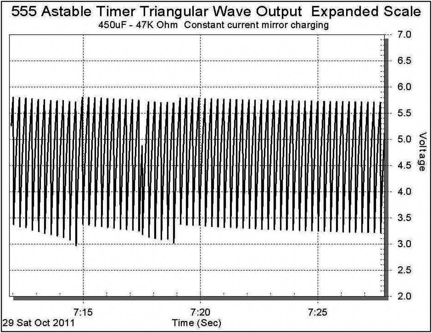
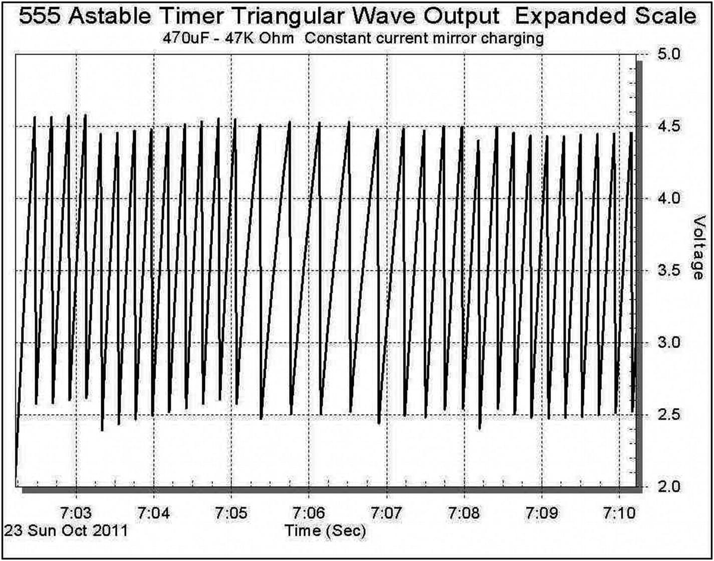
For slower signal changes, DAQFactory’s ability to store graphical data in its channels and then be able to display it as a strip chart recording can be very useful in revealing hidden information. If the triangular waveform of Figure 9-12 is recorded for 8 to 10 minutes and then the time scale of the graphical display is reconfigured to display an 8-minute window of the data (i.e., an 8-minute window would be 8 minutes × 60 = 480 for the time base), then a host of variations become evident, as displayed in Figures 9-24 and 9-25.
In Figures 9-24 and 9-25, extending the time scale over which the repetitive voltage cycles are displayed has brought out visually the influences of several ubiquitous experimental sources of error.
Most individuals are familiar with the propagation of water waves in a body of still water. Water waves from two sources caused by stones thrown into a pond appear to our eyes to pass through one another without interference. However, if an object is floating on the surface of the water at the same point where the waves pass through one another, a violent pitching of the object is seen. The violent pitching is caused by the superposition principle that sums the amplitudes of the two water displacement waves passing through one another. The distortions visible at 7:14:30 and 7:19:00 in Figure 9-24 could be caused by a second voltage variation wave with an amplitude of ½ volt and a frequency of one cycle in 4 1/2 minutes blending with or interfering with the main signal.
Long-Term Signal Distortions
The recorded triangular waveforms are reasonably reproducible with respect to their frequency of occurrence as the author’s breadboarded circuit can be seen to be producing 19 cycles in 5 minutes. The reproducibility of the voltage levels however can be seen to be both drifting and oscillating. The lower values for the voltage vary from 3.0 to 3.4, while the upper values vary from 5.7 to 5.0. Although the upper and lower voltage values are varying, the display has a distinct pattern that suggests the system is both drifting and oscillating due to the factors discussed previously.
Finger Heat Applied to Left Transistor of Current Mirror
Finger Heat Applied to Right Transistor of Current Mirror
The erratic amplitude seen in addition to the altered cycle time is also a result of thermal effects.
The materials from which electronic components are fabricated also contribute to the noise seen in electronic circuits. Wire-wound resistors are the least noisy, metal films are intermediate, and carbon-based components exhibit the greatest contribution to resistor circuit noise.
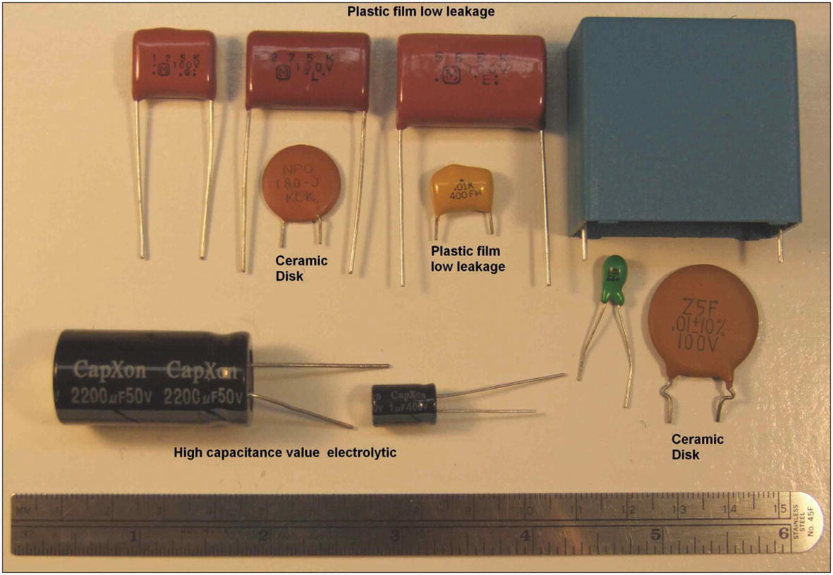
Various Types of Fixed Value Capacitors
Creation of a symmetrical triangular waveform can be done with op-amps and capacitors, but a circuit known as a voltage-controlled oscillator has been designed to simultaneously produce both square and symmetrical triangular waveforms. The Exar XR-2209 IC is a module that with an external capacitor and resistor can be powered by dual or single, 4- to +/–13-volt supplies to produce the required signal. Figures 9-16 and 9-17 are typical outputs from the IC. The triangular wave in the author’s breadboard setup can be seen to systematically vary in the peak voltages achieved. The breadboard setup also proved to be very sensitive to the value of the “pull-up” resistor used to develop the square waveform. The component sensitivity is probably due to operating the circuitry in an area near to the extremes of the circuit design.
X-Y Recordings
x-y recordings are often used when the signal to be recorded is cyclic in nature. Because of the cyclic nature of the signal, it is desirable to clear old traces from the x-y screen as new ones will be overlaid on the older data traces. By specifying the number of data points to plot, using the [n] channel value notation, any fraction or multiple of signal cycles can be displayed.
The effects of non-reproducible signals that are seen in Figures 9-22 and 9-23 arise from the same causes that are evident in the variations of the recorded x vs. time signals of Figures 9-24, 9-25, and 9-26.
Microcontroller Data Plotting
Programmable microcontrollers supported by open source, online communities are constantly having their base capabilities expanded, and a data plotting facility has been added to the Arduino IDE from version 1.6.6 onward.
In previous exercises, the Arduino microcontroller has been used as a smart data acquisition device, a power source for sensors or displays, and a clock; and in this chapter, it will be used to provide a visual graphical display of data.
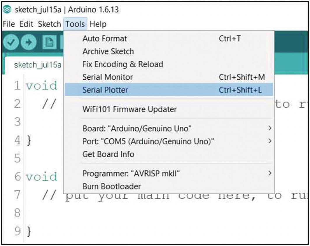
Arduino IDE Tools Menu Serial Plotter Selection
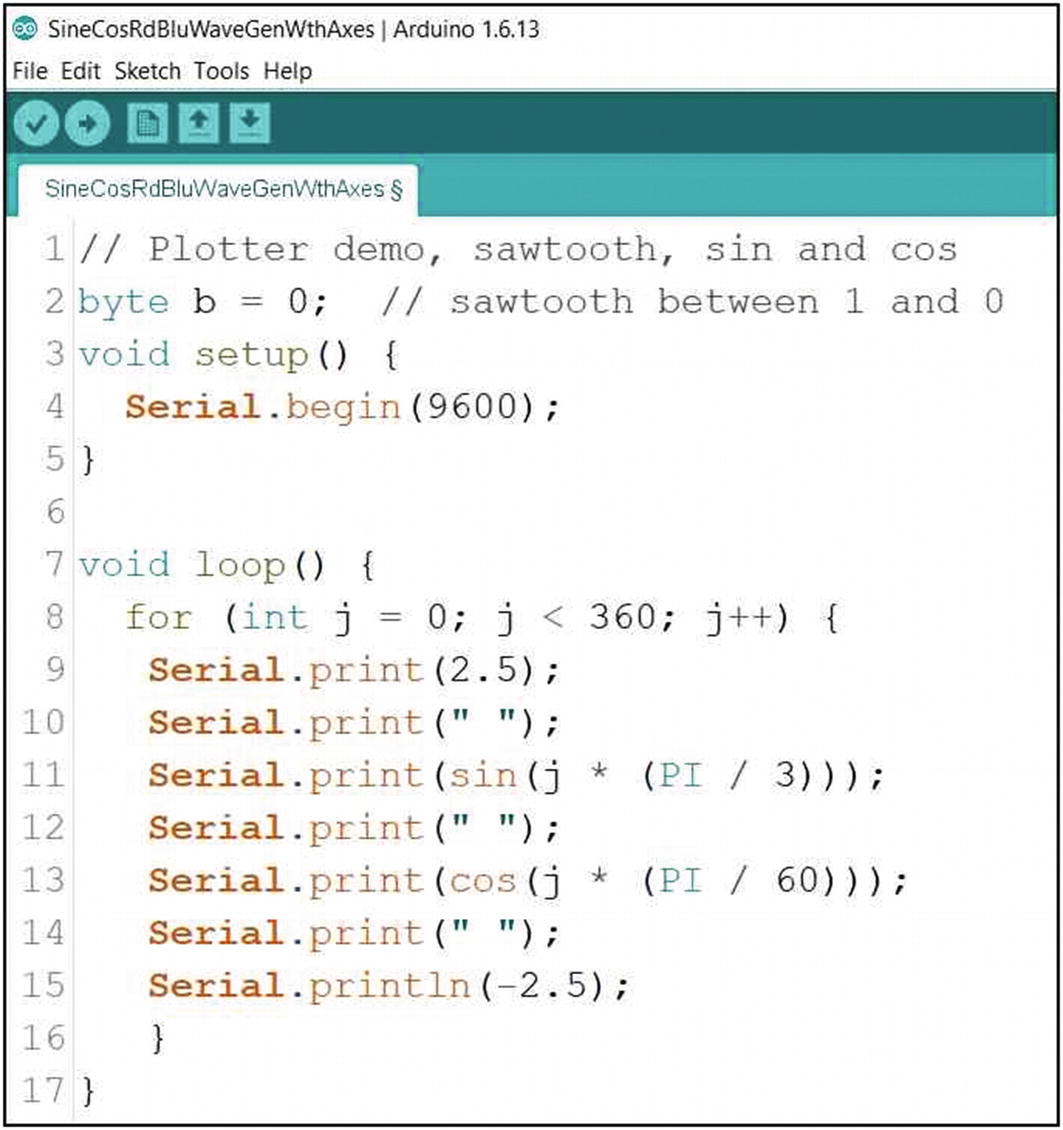
Invoking the serial plotter output converts the serial port window display into an x-y plotter. Individual data points directed to the serial port for display with a print statement are plotted on the vertical y axis. The x axis auto-scrolls from left to right in the form of a 500-point moving window. The metric for the x axis is the processing of the line of code with the line feed print instruction. Line 15 in Figure 9-29 contains the println code that is counted as processed and whose total value forms the numerical values displayed on the x axis.
For multiple-point plotting, each data value to display with a separate trace is separated from the next with either a print white space instruction or a tab instruction: ( print(“ “); or print(“/t);). Lines 10, 12, and 14 in Figure 9-29 form the separation markers for the four-trace plot seen in Figure 9-30.
Experimental
Observations

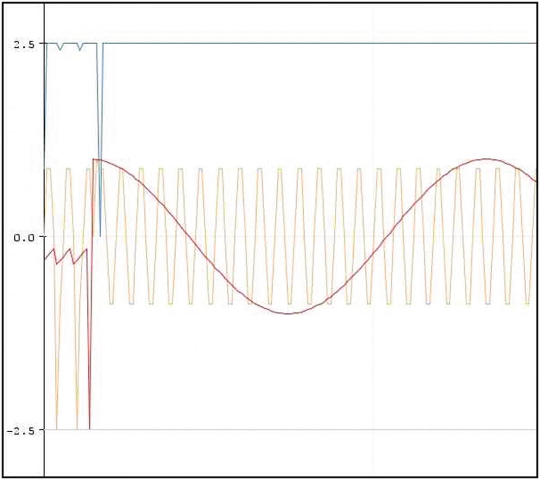
Arduino Serial Plotter Output
Examination of the microprocessor plotter demonstration code and the displayed frequencies of the sinusoids validates the expected 20:1 frequency ratio between the sine wave and cosine. The constant values plot as the expected straight lines.
Discussion
Inclusion of the plotter in the Arduino’s IDE has made a very powerful visualization technique available to the experimental investigator. The plotter is both very easy to use and useful. Plots generated by an experimental process being controlled by the microprocessor can be recorded for archiving with the print screen function available on host computers. Experimental plot archiving has been used in experimental work involving the measurements of temperature, motion, and vibration and in light and optics investigations.
Although the plotter is a very useful function, it is at the time of manuscript preparation limited in several aspects of operation. The colors of the traces are fixed by the operating system of the IDE and can be difficult to see at times. The scales are auto-adjusting and unlike the DAQFactory plotter cannot be independently set to different values.
Arduino Serial Plotter Start-Up Noise
As is seen in the preceding figure, the plotter settles into reproducibility reasonably quickly but on occasion may plot erroneously until the 500-point window refreshes itself and the auto-scale functions also settle into a reproducible plot mode.
Graphical Data Recording with Python and the Raspberry Pi
Introduction
As noted, graphical plotting of experimental data can take two forms. If the data is generated at a high rate, it is best saved by streaming into memory for storage and analyzed graphically at a later time. Experimental data generated at a slower rate can often be displayed as it is created in a “live” or “real-time” display. Python and the RPi use a graphical plotting library called matplotlib for display of both live and stored data.
An example of a Python matplotlib code that plots out the values of the voltage at the wiper arm of a 10 kΩ potentiometer biased between the 3.3-volt RPi power source on the GPIO array and its ground is provided in Listing 9-1 at the end of the chapter. The code has been modified from the strip chart recorder program that can be found as “animation example code: strip_chart_demo.py” in the matplotlib documentation. The documentation contains a full development tutorial for the use of this type of animated graphical display.
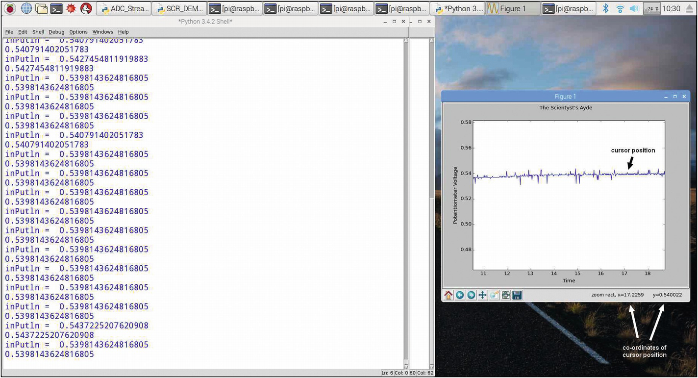
Although the RPi does not have an extensive selection of commercial graphical display software applications available, the matplotlib can provide a substantial basis from which the required application can be developed. The relatively short program used to monitor the varying potentiometer voltage in this exercise is equipped with several advanced utilities for in-depth examination of the recorded graphical presentation. A section of the matplotlib documentation entitled “Interactive Navigation” describes the actions of the seven buttons seen in the bottom-left corner of the plotting display as seen in Figures 9-32 and 9-34. The left button restores the focus of the display when any of the display manipulation or storage buttons has been used. Buttons allow sections of the recorded trace to be saved as seen in Figure 9-33 and enlarged as seen in Figures 9-34, 9-35, and 9-36. In addition to the button-activated utilities, the library example also displays the coordinates of the mouse cursor so that exact points can be identified by placing the cursor pointer at a point of interest in the tracing and reading the x and y coordinates of the point in terms of the display time and the measured data value from the numerical values displayed in the lower right-hand corner of the plotter frame.
The matplotlib program is also very easy to alter the scale of either plotting axis, but because of the time scale inconsistencies seen in previous exercises, the plotter time base displayed needs to be calibrated as described in the following experimental section.
Experimental
To demonstrate the plotting facility available with the RPi, an example can be created from the gpiozero library and an MCP3008 ADC IC reading the voltage from the wiper of a biased potentiometer. The wiper voltage is digitized by an MCP3008, 10-bit ADC configured as described in Chapter 6, Figure 6-17. To facilitate programming with the ADC, the gpiozero library has been used to provide the plotting data through accessing the “pot.value” attribute of the object instantiated in the line “pot = MCP3008(0)”. The creation of the pot object with the gpiozero library enables the programmer to access the wiper voltage value connected to the first channel on the ADC chip. The value is automatically normalized to a dimensionless floating-point value between 0 and 1 by setting the code variable to be plotted equal to the pot.value attribute.
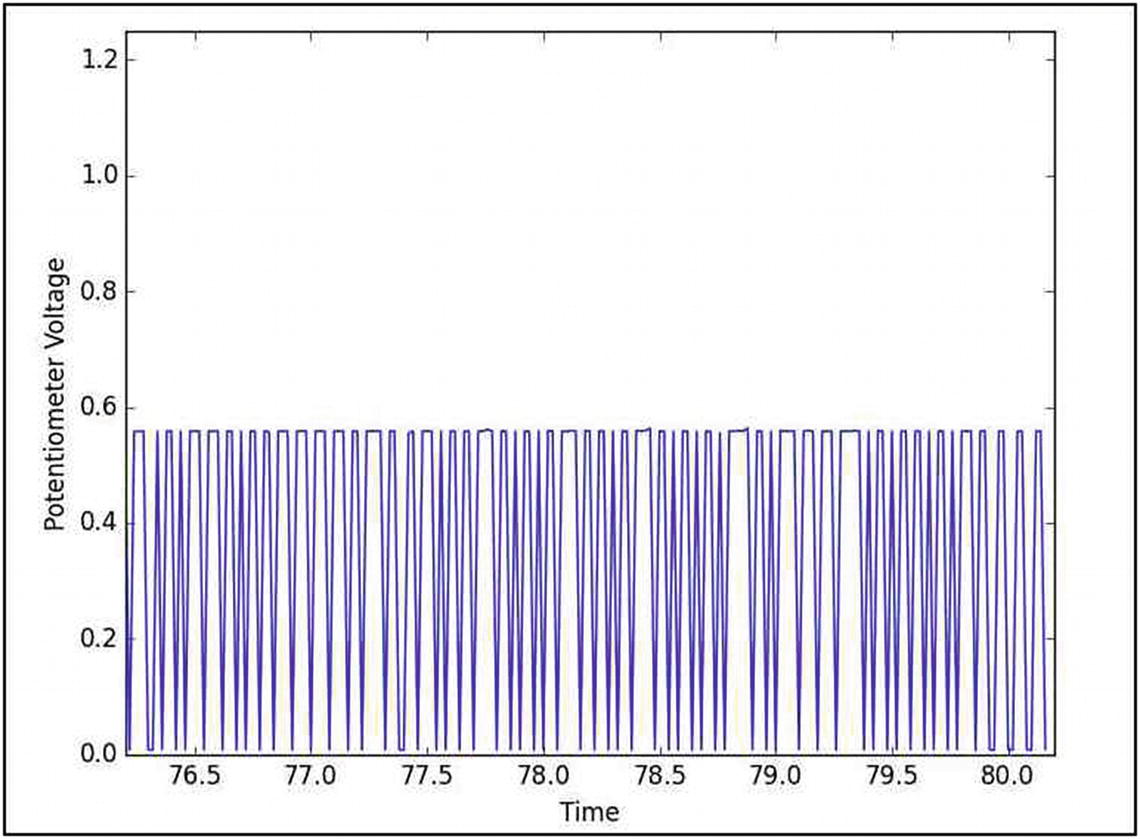
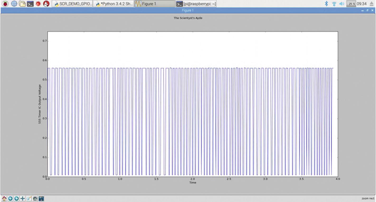
The configuration of the RPi with the gpiozero library to access the MCP3008 ADC also allows the plotting program to be modified to accept any sensor or transducer that is able to supply a voltage value of 3.3 V or less. Figures 35 and 36 are two traces that have been made from the output of a 555 IC timer that has been wired to the first or 0 channel of the digital converter. The configuration of the 555 IC is illustrated in the right-hand drawings and circuitry of Chapter 8, Figure 8-8. For this experiment, R1 and R2 were 4.7 kΩ, and C1 was a 100 μF electrolytic capacitor in the 555 timer RC network. The output circuitry also included an LED and current limiting resistor to aid in circuitry assembly, verification of electrical operation, and validation of recorder display by observing a continuous LED flashing at a rate of 59 flashes in 60 s. The final two expanded scale figures, Figures 9-37 and 9-38, were made with the “save a trace” button of the options row at the bottom left of the plotter display.
In order to aid in the development of the adaptation of the published matplotlib strip chart recorder code that uses an internal random number generator to create the y values for the plotter example output, the author inserted a number of diagnostic print statements in the code being modified. The print statements stream out the values of certain variables at points in the executing code to the Python console to aid in the development of different methods for adapting the code to follow data from different sources. Commenting out the diagnostic print lines will clear the console display. The streamed-out variable data is seen in the console displays as the left-hand screens in Figures 9-32 to 9-34. When no longer required, the print lines can be commented out.
Several factors must be taken into account when using graphical data displays on the RPi. As has been noted in previous exercises and previously, the time base of the system is not constant, and hence the time scale at the bottom of the plotter display is of limited reliability and must be semi-quantitatively calibrated for semi-quantitative use (see “Discussion”).
Adjusting Plotter Time Base
Dt Setting | Time Width (sec) |
|---|---|
0.02 | 25 |
0.01 | 41 |
0.005 | 127 |
0.0055 | 116 |
0.00525 | 129 |
0.005 | 125 |
Observations

A Data Recording of Potentiometer Wiper Voltage
Figure 9-32 displays the voltage value trace from 80 to 120 minutes into the experiment in which the author has manually turned the potentiometer shaft at the times recorded on the un-calibrated relative time axis of the display. The trace is relatively quick to respond, but rapid twisting of the shaft can overrun the display’s ability to keep up with the changing data value.

The “Save a Figure” Option Window
In the screen capture of Figure 9-34, the cursor of the mouse had been placed on the vertical response line just past 17 minutes, and the exact coordinates of the point were then printed in the bottom right-hand corner of the display.
The “Scale Expansion” Option
Expanded Time Scale 555 Timer Data Recording

One-Minute Time Scale Expansion of 555 Timer Data Recording
Discussion
Graphical data recording with the strip chart recorder program from the Python matplot library is a very adaptable and flexible system that can be used to display data directly from sensors attached to the GPIO array or from the Python serial port.
A Calibrated Time Base 555 Timer Voltage Output Recording
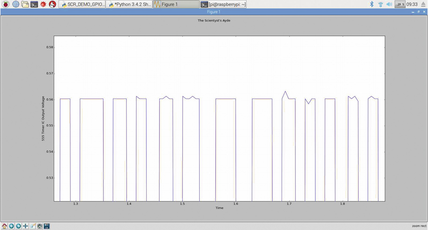
A Time-Calibrated Plotted Trace Expansion
A significant number of sensors have been coded into the gpiozero library that could be used to provide data for the matplotlib plotting program.
One of the advantages of graphical data displays becomes obvious when the variation in the time width of the rectangular pulses is presented in the visual format of Figure 9-38.
Table 9-1 demonstrates a limitation of the time base used for the RPi graphical data displays. A progressive incremental halving of the Dt value increased the time measurement, but the return to the 0.005 value produced a 2-second difference from the original measured value. The differential validates the earlier caution noted in the manuscript with respect to the RPi operating system priorities that can interfere with the timekeeping of the input and output operations of the computer.
Code Listing
Python Code for Live or Real-Time Data Plotting with Raspberry Pi
Summary
Experimental data recorded graphically as a plotting of y vs. time or as x vs. y can show numerous electronically generated waveforms and sensor readouts.
Graphical data recordings can reveal signal drifting and signal deviations and display electrical, mechanical, and environmental influences on signal outputs not normally visible in numeric displays.
Commercial SCADA plotting is easily configured, robust, and very flexible, while component-assembled systems are more constrained in display capability and must be calibrated manually.
In Chapter 10, various methods of current control, an important aspect of experimental equipment configurations or design, are presented.