
CHAPTER 13
Forecasting
THE CHALLENGE
Mean-variance analysis requires investors to specify views for expected returns, standard deviations, and correlations. These properties of assets vary over time. Long-run averages are poor forecasts because they fail to capture this time variation. On the other hand, extrapolating from a short sample of recent history is ineffective because it introduces noise and assumes a level of persistence that does not occur reliably (see Chapter 19 on estimation error, and Chapter 9 on the fallacy of 1/N). As an alternative, investors may use additional data such as economic variables to project expected returns from the current values of those variables and their historical relationships to asset returns. However, this approach does not guarantee success because additional variables contribute noise along with information. The investor's challenge is to maximize the information content and minimize the noise, thereby generating the most effective predictions. In this chapter, we reinterpret linear regression to reveal the predictive information that comes from each historical observation in our sample, and we extend it to focus on a subset of the most relevant historical observations, which can significantly improve the quality of the forecasts. This procedure, which was introduced by Czasonis, Kritzman, and Turkington (2020), is called partial sample regression.
CONVENTIONAL LINEAR REGRESSION
Financial analysts face the challenge of mapping predictive variables onto the assets they want to forecast. The goal is to identify relationships from history that are likely to apply in the future. Let us begin by reviewing one of the most common forecasting techniques: linear regression. It assumes that the variable we are trying to predict,
![]() , is a linear function of a set of predictive variables,
, is a linear function of a set of predictive variables,
![]() (a row vector), plus an error term,
(a row vector), plus an error term,
![]() :
:
The simplicity of the linear model is attractive. Compared to a more complex model, it is less likely to overfit the data and identify spurious relationships. To find the vector of coefficients,
![]() (a column vector), we solve for the values that minimize the sum of squared prediction errors between the model's forecasts,
(a column vector), we solve for the values that minimize the sum of squared prediction errors between the model's forecasts,
![]() , and the actual values of the dependent variable:
, and the actual values of the dependent variable:
This method is called Ordinary Least Squares (OLS). It is quite like the portfolio optimization method we describe in Chapter 2, where we minimize risk as the sum of squared deviations of portfolio returns from their average. The solution to the linear regression problem is shown in matrix notation as follows:
![]() is the best linear unbiased estimate of the variable coefficients, which means they extract information from the data set as efficiently as possible, given their intended goal. To arrive at a forecast of the dependent variable, we multiply each variable in the
is the best linear unbiased estimate of the variable coefficients, which means they extract information from the data set as efficiently as possible, given their intended goal. To arrive at a forecast of the dependent variable, we multiply each variable in the
![]() vector by its estimated coefficient in
vector by its estimated coefficient in
![]() and compute the sum, which in matrix notation is
and compute the sum, which in matrix notation is
Linear regression is a statistically robust process that performs well in many applications, but it has two important shortcomings. First, its traditional interpretation in terms of the relative importance of each variable does not match the way people intuitively extrapolate from past events, so it can be hard to reconcile model outputs with our judgment. Second, it does not capture nonlinear or conditional relationships between variables.
Next, we present a solution to these shortcomings. We show that by reinterpreting regression predictions as a weighted sum across observations – rather than a weighted sum across variable values – we align intuition with the way we naturally extrapolate from events. This insight leads to a new set of models called partial sample regressions, whereby omitting less relevant observations can substantially improve the quality of our forecasts.
REGRESSION REVISITED
Let us now approach the prediction challenge from a different perspective. Imagine we are given a set of historical observations for predictive variables,
![]() (a matrix of stacked time observations), and a prediction target,
(a matrix of stacked time observations), and a prediction target,
![]() , and we are asked to generate a forecast for
, and we are asked to generate a forecast for
![]() in the future based on current values for
in the future based on current values for
![]() . How might we proceed?
. How might we proceed?
One intuitive approach is to begin by measuring the similarity of each historical observation
![]() , to today,
, to today,
![]() . We define multivariate similarity as the opposite (negative) of the Mahalanobis distance between the two points. It is also multiplied by 1/2 to compensate for the fact that
. We define multivariate similarity as the opposite (negative) of the Mahalanobis distance between the two points. It is also multiplied by 1/2 to compensate for the fact that
![]() and
and
![]() are compared twice by the multiplications in the formula. The Mahalanobis distance (as described in Chapter 25) represents the distance between two vectors as a function of the normalized distances between the respective elements of the vectors as well as the degree to which co-movement across variables is unusual. The larger the distance, the less similar two observations are, and vice versa.
are compared twice by the multiplications in the formula. The Mahalanobis distance (as described in Chapter 25) represents the distance between two vectors as a function of the normalized distances between the respective elements of the vectors as well as the degree to which co-movement across variables is unusual. The larger the distance, the less similar two observations are, and vice versa.
Here,
![]() is the inverse of the covariance matrix of the variables in
is the inverse of the covariance matrix of the variables in
![]() . (Note that we use
. (Note that we use
![]() to denote the covariance matrix in other chapters, but we use the symbol
to denote the covariance matrix in other chapters, but we use the symbol
![]() in this chapter to avoid confusion with summation operators in the formulas that follow.) All else being equal, similarity is higher when the values in
in this chapter to avoid confusion with summation operators in the formulas that follow.) All else being equal, similarity is higher when the values in
![]() and
and
![]() are closer to each other, and when the deviations in values align with common patterns for the variables. For example, if economic growth and inflation are positively correlated, a deviation of both variables in the same direction would not increase the distance by much, but a deviation in the opposite direction would. It is reasonable to think that in the next period,
are closer to each other, and when the deviations in values align with common patterns for the variables. For example, if economic growth and inflation are positively correlated, a deviation of both variables in the same direction would not increase the distance by much, but a deviation in the opposite direction would. It is reasonable to think that in the next period,
![]() might behave the same way it has behaved following similar periods in history. This is certainly more intuitive than predicting that y will behave as it has behaved following the most different periods in history.
might behave the same way it has behaved following similar periods in history. This is certainly more intuitive than predicting that y will behave as it has behaved following the most different periods in history.
What if there are two historical events that are equally like today, but different from each other? Suppose that one such observation is closer to the long-run mean than
![]() , whereas the other is farther from the mean. Which of these observations contains better information for predicting
, whereas the other is farther from the mean. Which of these observations contains better information for predicting
![]() ? The answer is that we should rely more on the unusual observation and less on the typical one, because the unusual observation likely contains more event-driven information, whereas the typical observation more likely reflects noise. Following this intuition, we measure the informativeness of each observation as its Mahalanobis distance from the long-run average of
? The answer is that we should rely more on the unusual observation and less on the typical one, because the unusual observation likely contains more event-driven information, whereas the typical observation more likely reflects noise. Following this intuition, we measure the informativeness of each observation as its Mahalanobis distance from the long-run average of
![]() . We scale it by 1/2 as we did for similarity.
. We scale it by 1/2 as we did for similarity.
Together, similarity and informativeness tell us the relevance of each historical observation. Similarity compares each observation to the one we are using to forecast, whereas informativeness compares each observation to the average across the entire data set:
To build intuition for the measure of relevance, let us consider some examples. If a historical observation “A” is identical to
![]() , the distance between them is zero, so A's similarity is as high as possible (similarity becomes less and less negative as distance falls). Therefore, A's relevance score equals its informativeness. All other observations must have a lower (more negative) similarity to
, the distance between them is zero, so A's similarity is as high as possible (similarity becomes less and less negative as distance falls). Therefore, A's relevance score equals its informativeness. All other observations must have a lower (more negative) similarity to
![]() . If observation B is as informative as A but less similar to
. If observation B is as informative as A but less similar to
![]() , it has lower relevance for our forecast. The historical
, it has lower relevance for our forecast. The historical
![]() value corresponding to B may help our prediction, but we should put less weight on it than A. An observation with low similarity, low informativeness, or both, could have a relevance of zero. We would ignore the y value that corresponds to this observation.
value corresponding to B may help our prediction, but we should put less weight on it than A. An observation with low similarity, low informativeness, or both, could have a relevance of zero. We would ignore the y value that corresponds to this observation.
What does it mean if relevance is negative?1 This is often the case. It occurs for historical observations that are informative in their own right, but also very different from
![]() . For example, if
. For example, if
![]() reflects robust economic growth, historical data from a severe recession probably has negative relevance. We might assume that such points are so different from
reflects robust economic growth, historical data from a severe recession probably has negative relevance. We might assume that such points are so different from
![]() that we should predict the opposite of the
that we should predict the opposite of the
![]() values that correspond to them. Amazingly, it turns out that if we multiply each historical value of
values that correspond to them. Amazingly, it turns out that if we multiply each historical value of
![]() by that period's relevance and average the results, we end up with precisely the linear regression forecast. The following equations demonstrate this equivalence. For notational convenience and without loss of generality, we assume that all
by that period's relevance and average the results, we end up with precisely the linear regression forecast. The following equations demonstrate this equivalence. For notational convenience and without loss of generality, we assume that all
![]() and
and
![]() variables are shifted to have means of zero.
variables are shifted to have means of zero.
Because the average of
![]() is zero:
is zero:
In Equation 13.17, beta is the vector of coefficients from a traditional linear regression. Table 13.1 shows this equivalence for a simplified example with only one independent variable and samples for
![]() and
and
![]() that have means of zero. It is straightforward to expand to multiple variables and nonzero means,
that have means of zero. It is straightforward to expand to multiple variables and nonzero means,
![]() , using the following formula:
, using the following formula:
TABLE 13.1 Equivalence of Prediction from Linear Regression and Relevance-Weighted Dependent Variable
| Traditional calculation | Relevance-weighted calculation | ||||||
|---|---|---|---|---|---|---|---|
| Observation | X (%) | Y (%) | Similarity (to X = 10%) | Informativeness | Relevance | Scaled Y values (%) | |
| 1 | −15 | −10 | −6.25 | 2.25 | −4.00 | 20 | |
| 2 | −5 | −20 | −2.25 | 0.25 | −2.00 | 20 | |
| 3 | 0 | 10 | −1.00 | 0.00 | −1.00 | −5 | |
| 4 | 5 | 0 | −0.25 | 0.25 | 0.00 | 0 | |
| 5 | 15 | 20 | −0.25 | 2.25 | 2.00 | 20 | |
| Slope: | 1.1 | Average: | 11% | ||||
| Prediction for X = 10% | 11% | ||||||
In summary, we presume that more similar observations are more relevant, and that more informative observations are more relevant, all else being equal. We combine these two scores and apply the result as a “weight” to each historical observation of the dependent variable we wish to forecast. Summing across all observations produces the same forecast as linear regression. Viewed this way, it is interesting to note that to predict different
![]() variables we need only replace the dependent variable observations while retaining the same historical relevance scores.
variables we need only replace the dependent variable observations while retaining the same historical relevance scores.
How Many Anecdotes Do We Need?
It is often said that the plural of “anecdote” is “data.” Our observation-based perspective of regression analysis illustrates this point. If we include only the single most relevant observation, our forecast is that whatever happened at that time will reoccur. This forecast comes from the most relevant possible data, but it is noisy because it extrapolates from a single event. If instead we include every observation, our forecast aggregates across the full extent of available data. This forecast is statistically robust, but it may reflect noise from less-relevant observations. Most notably, it assumes that what happened during the most dissimilar historical periods will reoccur but in the opposite direction. For these bets to work, we need perfect symmetry. This is the essence of “linearity” in a linear model. It is not necessarily intuitive and may provide a poor description of the real world. For example, does it make more sense to predict health outcomes for a young, athletic woman from a data sample of her peers, or by predicting the opposite of what happens to old men with sedentary lifestyles?
We might decide to disregard data that are sufficiently irrelevant. The good news is that building a model with this sophistication is not difficult. All we need to do is censor the least relevant observations and form predictions from the remaining observations. This approach is called partial sample regression.
PARTIAL SAMPLE REGRESSION
In partial sample regression, we average over a subset of
![]() observations, rather than the full data set
observations, rather than the full data set
![]() . With this change, we must generalize our previous formula for relevance-weighted observations in two ways. The final prediction formula is
. With this change, we must generalize our previous formula for relevance-weighted observations in two ways. The final prediction formula is
In Equation 13.19, the mean is also computed on the relevant subsample
![]() . This formula converges to two intuitive edge cases. If we include all N observations, the estimate is equal to that of a standard linear regression. If we include only a single data point
. This formula converges to two intuitive edge cases. If we include all N observations, the estimate is equal to that of a standard linear regression. If we include only a single data point
![]() that is precisely equal to
that is precisely equal to
![]() , the prediction equals
, the prediction equals
![]() for that observation.
for that observation.
Comparison to Other Approaches
Partial sample regression may be viewed as an application of “kernel regression,” which extrapolates from near-neighbors of each observation, but it includes two essential distinguishing features. First, using the Mahalanobis distance to assess similarity is not an arbitrary choice, but is motivated by the rigor of OLS linear regression. Second, we consider informativeness in addition to similarity.
Partial sample regression is also distinct from other common variants of linear regression. For example, we cannot simply perform a new linear regression on the filtered subsample of data. The new regression would implicitly compute new relevance scores that systematically underestimate true relevance and therefore bias the results, because it is not aware that we already restricted attention to a subset of highly relevant observations. Partial sample regression is also quite different from weighted least squares. Weighted least squares applies weights to observations before evaluating their covariances, whereas partial sample regression filters the observations after the covariance matrix has already been computed.
Of course, there are endless possibilities for complex models to capture the complex relationships of assets and predictive variables. The relative simplicity of partial sample regression, combined with its ability to detect conditional relationships, is its main advantage.
Predicting Returns of Factors and Asset Classes
Partial sample regression is a general approach that may be used to forecast anything. It provides statistical rigor along with intuitive appeal. Whether or not its forecasts are more reliable than those from other models is an empirical question. In practice, we find that it often performs better than traditional linear regression. In this section, we illustrate its value for predicting the returns of asset classes and factors from economic variables. (In Chapter 14, we apply it to forecasting the correlation between stocks and bonds.)
We use the following US economic data, each of which is computed as a year-over-year percentage change for a sequence of three consecutive years, as our
![]() variables, in order to measure the relevance of the historical observations:
variables, in order to measure the relevance of the historical observations:
- Industrial production
- Inflation
As Y variables, we consider the following asset classes and factor premiums (the five factors proposed by Fama and French [2015] plus the traditional stock momentum factor) for the US market:
- Equities minus cash
- Government bonds minus cash
- Corporate bonds minus government bonds
- Commodities minus cash
- Small minus large stocks
- Value minus growth stocks
- High minus low profitability stocks
- High minus low investment stocks
- Positive minus negative momentum stocks
For a given prediction, we compute the relevance of each historical observation and identify the top 25%. First, let us consider a prediction that one might make as of mid-2020, using available observations for 2018 and 2019 and hypothesizing values for the full year of 2020. Specifically, let us assume that industrial production over these three years is 2.0%, 1.8%, and −6.0%, and that inflation is 1.9%, 2.3%, and 1.0%. Figure 13.1 shows the relevance of each historical three-year path together with the equity risk premium that prevailed in the following year.
Partial sample regression amounts to weighting the dependent variable observations in Figure 13.2 by their relevance and averaging them. In this example, the forecast for the equity risk premium conditional on the economic path we specified is 10.9%.
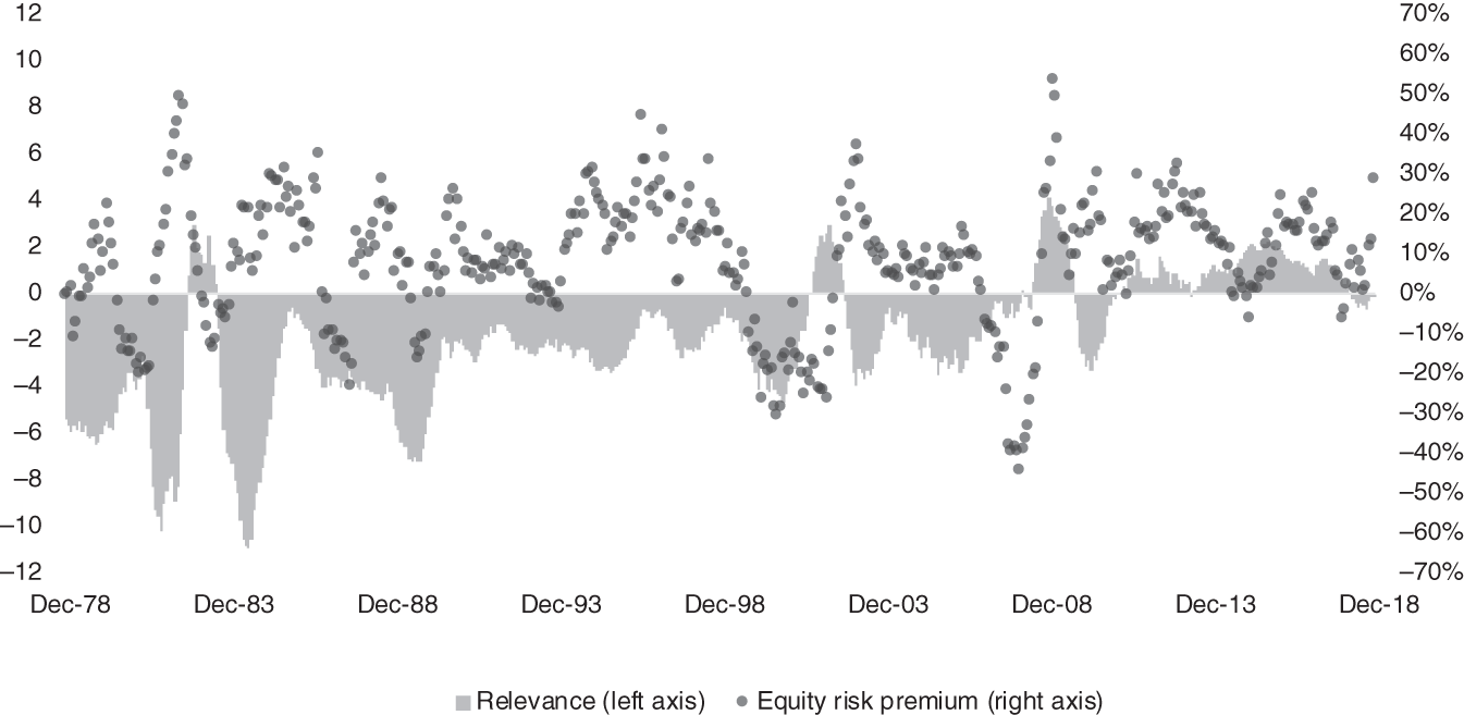
FIGURE 13.1 Relevance and dependent variable values for a sample input.

FIGURE 13.2 The most relevant observations.
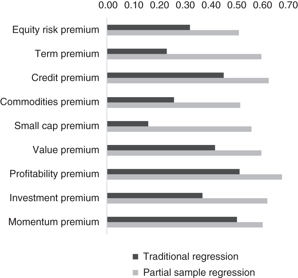
FIGURE 13.3 Prediction efficacy for partial sample regression versus traditional linear regression (correlation of predicted and realized values).
Next, we repeat this prediction process for each historical observation in our data set, and for each asset class and factor premium. We then evaluate the correlation between predictions and actual occurrences of the dependent variable. Figure 13.3 shows that the correlation between predicted and realized values increases substantially in every case.
THE BOTTOM LINE
Investors may wish to adjust their portfolios as conditions change. An effective process requires accurate forecasts for expected returns, standard deviations, and correlations. Although some investors may choose to rely on qualitative judgment, others may prefer to use historical data as a guide. Naïve extrapolation of previous returns does not usually work well. Instead, investors can relate asset performance to a set of predictive variables. The analytical process becomes more intuitive when we reinterpret linear regression as a relevance-weighted average over historical observations. With this approach, it is often possible to improve forecasts by simply eliminating a portion of the less-relevant information.
RELATED TOPICS
- Chapter 9 discusses the importance of using reasonable expected returns as inputs to portfolio optimization.
- Chapter 14 applies partial sample regression to forecast the correlation between stocks and bonds.
REFERENCES
- Czasonis, M., Kritzman, M., and Turkington, D. 2020. “Addition by Subtraction: A Better Way to Predict Factor Returns (and Everything Else),” The Journal of Portfolio Management, Vol. 46, No. 8 (September).
- Fama, E. F. and French, K. R. 2015. “A Five Factor Asset Pricing Model,” Journal of Financial Economics, Vol. 116, No. 1 (April).
NOTE
- 1. To be precise, interpreting the sign of an observation’s relevance requires that we center relevance around zero by subtracting its average value (which will be negative), or equivalently that we augment the definition of relevance with the addition of the informativeness of xt. Adding any constant to all of the relevance terms has no effect on the prediction because it amounts to a constant times the sum of deviations of Y, which is zero.