Chapter 2: Automated Machine Learning, Algorithms, and Techniques
Automating the automation sounds like one of those wonderful Zen meta ideas, but learning to learn is not without its challenges. In the last chapter, we covered the Machine Learning (ML) development life cycle, and defined automated ML, with a brief overview of how it works.
In this chapter, we will explore under-the-hood technologies, techniques, and tools used to make automated ML possible. Here, you will see how AutoML actually works, the algorithms and techniques of automated feature engineering, automated model and hyperparameter turning, and automated deep learning. You will learn about meta-learning as well as state-of-the-art techniques, including Bayesian optimization, reinforcement learning, evolutionary algorithms, and gradient-based approaches.
In this chapter, we will cover the following topics:
- Automated ML – Opening the hood
- Automated feature engineering
- Hyperparameter optimization
- Neural architecture search
Automated ML – Opening the hood
To oversimplify, a typical ML pipeline comprises data cleaning, feature selection, pre-processing, model development, deployment, and consumption steps, as seen in the following workflow:
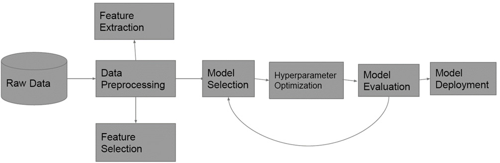
Figure 2.1 – The ML life cycle
The goal of automated ML is to simplify and democratize the steps of this pipeline so that it is accessible by citizen data scientists. Originally, the key focus of the automated ML community was model selection and hyperparameter tuning, that is, finding the best-performing model for the job and the corresponding parameters that work best for the problem. However, in recent years, it has been shifted to include the entire pipeline as shown in the following diagram:
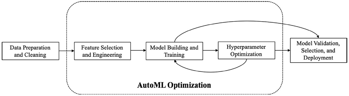
Figure 2.2 – A simplified AutoML pipeline by Waring et al.
The notion of meta-learning, that is, learning to learn, is an overarching theme in the automated ML landscape. Meta-learning techniques are used to learn optimal hyperparameters and architectures by observing learning algorithms, similar tasks, and those from previous models. Techniques such as learning task similarity, active testing, surrogate model transfer, Bayesian optimization, and stacking are used to learn these meta-features to improve the automated ML pipeline based on similar tasks; essentially, a warm start. The automated ML pipeline function does not really end at deployment – an iterative feedback loop is required to monitor the predictions that arise for drift and consistency. This feedback loop ensures that the outcome distribution of prediction matches the business metrics, and that there are anomalies in terms of hardware resource consumption. From an operational point of view, the logs of errors and warnings, including custom error logs, are audited and monitored in an automated manner. All these best practices also apply to the training cycle, where the concept drift, model drift, or data drift can wreak havoc on your predictions; heed the caveat emptor warning.
Now, let's explore some of the key automated ML terms you will see in this and future chapters.
The taxonomy of automated ML terms
For newcomers to automated ML, one of the biggest challenges is to become familiar with the industry jargon – large numbers of new or overlapping terminologies can overwhelm and discourage those exploring the automated ML landscape. Therefore, in this book we try to keep things simple and generalize as much as possible without losing any depth. You will repeatedly see in this book, as well as in other automated ML literature, the emphasis being placed on three key areas – namely, automated feature engineering, automated hyperparameter turning, and automated neural architecture search methods.
Automated feature engineering is further classified into feature extraction, selection, and generation or construction. Automated hyperparameter tuning, or the learning of hyperparameters for a specific model, sometimes gets bundled with learning the model itself, and hence becomes part of a larger neural architecture search area. This approach is known as the Full Model Selection (FMS) or Combined Algorithm Selection and Hyperparameter (CASH) optimization problem. Neural architecture search is also known as automated deep learning (abbreviated as AutoDL), or simply architecture search. The following diagram outlines how data preparation, feature engineering, model generation, and evaluation, along with their subcategories, become part of the larger ML pipeline:
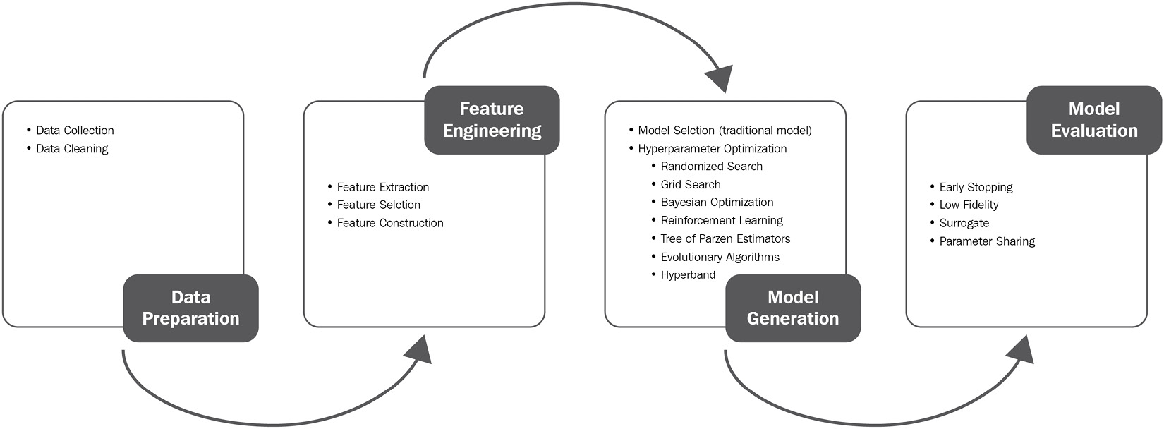
Figure 2.3 – Automated ML pipeline via state-of-the-art AutoML survey, He, et al., 2019
The techniques used to perform these three key tenets of automated ML have a few things in common. Bayesian optimization, reinforcement learning, evolutionary algorithms, gradient-free, and gradient-based approaches are used in almost all these different areas, with variations as shown in the following diagram:

Figure 2.4 – Automated ML techniques
So, you may get perplexed looks if you refer to using genetic programming in automated feature engineering, while someone considers evolutionary hierarchical ML systems as a hyperparameter optimization algorithm. That is because you can apply the same class of techniques, such as reinforcement learning, evolutionary algorithms, gradient descent, or random search, to different parts of automated ML pipelines, and that works just fine.
We hope that the information provided between Figure 2.2 and Figure 2.4 help you to understand the relationship between ML pipelines, automated ML salient traits, and techniques/algorithms used to achieve those three key characteristic traits. The mental model you will build in this chapter will go a long way, especially when you encounter preposterous terms coined by marketing (yes Todd, I am talking about you!), such as deep-learning-based-hyperparameter-optimization-product-with-bitcoins-and-hyperledger.
The next stop is automated feature engineering, the first pillar of the automated ML pipeline.
Automated feature engineering
Feature engineering is the art and science of extracting and selecting the right attributes from the dataset. It is an art because it not only requires subject matter expertise, but also domain knowledge and an understanding of ethical and social concerns. From a scientific perspective, the importance of a feature is highly correlated with its resulting impact on the outcome. Feature importance in predictive modeling measures how much a feature influences the target, hence making it easier in retrospect to assign ranking to attributes with the most impact. The following diagram explains how the iterative process of automated feature generation works, by generating candidate features, ranking them, and then selecting the specific ones to become part of the final feature set:

Figure 2.5 – Iterative feature generation process by Zoller et al. Benchmark and survey of automated ML frameworks, 2020
Extracting a feature from the dataset requires the generation of categorical binary features based on columns with multiple possible values, scaling the features, eliminating highly correlated features, adding feature interactions, substituting cyclic features, and handling data/time scenarios. Date fields, for instance, result in several features, such as year, month, day, season, weekend/weekday, holiday, and enrollment period. Once extracted, selecting a feature from a dataset requires the removal of sparse and low variance features, as well as applying dimensionality reduction techniques such as Principal Component Analysis (PCA) to make the number of features manageable. We will now investigate hyperparameter optimization, which used to be a synonym for automated ML, and is still a fundamental entity in the space.
Hyperparameter optimization
Due to its ubiquity and ease of framing, hyperparameter optimization is sometimes regarded as being synonymous with automated ML. Depending on the search space, if you include features, hyperparameter optimization, also dubbed hyperparameter tuning and hyperparameter learning, is known as automated pipeline learning. All these terms can be bit daunting for something as simple as finding the right parameters for a model, but graduating students must publish, and I digress.
There are a couple of key points regarding hyperparameters that are important to note as we look further into these constructs. It is well established that the default parameters are not optimized. Olson et al., in their NIH paper, demonstrated how the default parameters are almost always a bad idea. Olson mentions that "Tuning often improves an algorithm's accuracy by 3–5%, depending on the algorithm…. In some cases, parameter tuning led to CV accuracy improvements of 50%." This was observed in Cross-validation accuracy improvement – Data-driven advice for applying ML to bioinformatics problems, by Olson et al.: https://www.ncbi.nlm.nih.gov/pmc/articles/PMC5890912/.
The second important point is that a comparative analysis of these models leads to greater accuracy; as you will see in forthcoming chapters, the entire pipeline (model, automated features, hyperparameters) are all key to getting the best accuracy trade-off. The Heatmap for comparative analysis of algorithms section in Data-driven advice for applying ML to bioinformatics problems, by Olson et al. (https://www.ncbi.nlm.nih.gov/pmc/articles/PMC5890912/) shows the experiment performed by Olson et al., where 165 datasets were used against multiple different algorithms to determine the best accuracy, ranked from top to bottom based on performance. The takeaway from this experiment is that no single algorithm can be considered best-performing across all the datasets. Therefore, there is a definite need to consider different ML algorithms when solving these data science problems.
Let's do a quick recap of what the hyperparameters are. Each model has its internal and external parameters. Internal parameters or model parameters are intrinsic to the model, such as weight or the predictor matrix, while external parameters also known as hyperparameters, are "outside" the model; for example learning rate and the number of iterations. For instance in k-means, k stands for the number of clusters required and epochs are used to specify the number of passes done over the training data. Both of these are examples of hyperparameters, that is, parameters that are not intrinsic to the model itself. Similarly, the learning rate for training a neural network, C and sigma for Support Vector Machines (SVMs), k number of leaves or depth of a tree, latent factors in a matrix factorization, the number of hidden layers in a deep neural network, and so on are all examples of hyperparameters.
To find the correct hyperparameters, there are a number of approaches, but first let's see what different types of hyperparameters there are. Hyperparameters can be continuous, for example:
- The learning rate of a model
- The number of hidden layers
- The number of iterations
- Batch size
Hyperparameters can also be categorical, for example, the type of operator, activation function, or the choice of algorithm. They can also be conditional, for example, selecting the convolutional kernel size if a convolutional layer is used, or the kernel width if a Radial Basis Function (RBF) kernel is selected in an SVM. Since there are multiple types of hyperparameters, there are also a variety of hyperparameter optimization techniques. Grid, random search, Bayesian optimization, evolutionary techniques, multi-arm bandit approaches, and gradient descent-based techniques are all used for hyperparameter optimization:

Figure 2.6 – Grid and random search layout. Bergstra and Bengio – JMLR 2012
The simplest techniques for hyperparameter tuning are manual, grid, and random search. Manual turning, as the name suggests, is based on intuition and guessing based on past experiences. Grid search and random search are slightly different, as you pick a set of hyperparameters either for each combination (grid), or randomly and iterate through to keep the best performing ones. However, as you can imagine, this can get computationally out of hand quickly as the search space gets bigger.
The other prominent technique is Bayesian optimization, in which you start with a random combination of hyperparameters and use it to construct a surrogate model. Then you use this surrogate model to predict how other combinations of hyperparameters would work. As a general principle, Bayesian optimization builds a probability model to minimize the objective's function, using past performance to select the future values, and that is exactly what's Bayesian about it. As known in the Bayesian universe, your observations are less important than your prior belief.
The greedy nature of Bayesian optimization is controlled by exploration and exploitation trade-off (expected improvement), allocating fixed-time evaluations, setting thresholds, and suchlike. There are variations of these surrogate models that exist, such as random forest surrogate and gradient boosting surrogate, which use the aforementioned techniques to minimize the surrogate's function:

Figure 2.7 – A taxonomy of hyperparameter optimization techniques, Elshawi et al., 2019
The class of population-based methods (also called meta-heuristic techniques or optimization from samples methods) is also widely used to perform hyperparameter tuning, with genetic programming (evolutionary algorithms) being the most popular, where hyperparameters are added, mutated, selected, crossed over, and tuned. A particle swarm moves toward the best individual configurations when the configuration space is updated at each iteration. On the other hand, evolutionary algorithms work by maintaining a configuration space, and improve it by making smaller changes and combining individual solutions to build a new generation of hyperparameter configuration. Let's now explore the final piece of the automated ML puzzle – neural architecture search.
Neural architecture search
Selecting models can be challenging. In the case of regression, that is, predicting a numerical value, you have a choice of linear regression, decision trees, random forest, lasso versus ridge regression, k-means elastic net, gradient boosting methods, including XGBoost, and SVMs, among many others.
For classification, that in other words, separating out things by classes, you have logistic regression, random forest, AdaBoost, gradient boost, and SVM-based classifiers at your disposal.
Neural architecture has the notion of search space, which defines which architectures can be used in principle. Then, a search strategy must be defined that outlines how to explore using the exploration-exploitation trade-off. Finally, there has to be a performance estimation strategy, which estimates the candidate's performance. This includes training and validation of the architecture.
There are several techniques for performing the exploration of search space. The most common ones include chain structured neural networks, multi-branch networks, cell-based search, and optimizing approaches using existing architecture. Search strategies include random search, evolutionary approaches, Bayesian optimization, reinforcement learning, and gradient-free versus gradient-based optimization approaches, such as Differentiable Architecture Search (DARTS). The search strategy to hierarchically explore the architectural search spaces, using Monte Carlo tree search or hill climbing, is popular as it helps discover high-quality architectures by rapidly approaching better performing architectures. These are the gradient "free" methods. In gradient-based methods, the underlying assumption of a continuous search space facilitates DARTS, which, unlike traditional reinforcement learning or evolutionary search approaches, explores the search space using gradient descent. A visual taxonomy of neural architectural search can be seen in the following diagram:

Figure 2.8 – A taxonomy of neural architecture search techniques, Elshawi et al., 2019
To evaluate which approach works best for the specific dataset, the performance estimation strategies have a spectrum of simple to more complex (albeit optimized) approaches. Simplest among the estimation strategies is to just train the candidate architecture and evaluate its performance on test data – if it works out, great. Otherwise, toss it out and try a different architectural combination. This approach can quickly become prohibitively resource-intensive as the number of candidate architectures grows; hence, the low-fidelity strategies, such as shorter training times, subset training, and fewer filters per layer are introduced, which are not nearly as exhaustive. Early stopping, in other words, estimating an architecture's performance by extrapolating its learning curve, is also a helpful optimization for such an approximation. Morphing a trained neural architecture, and one-short searches treating all architectures as a subgraph of a super graph, are also effective approaches as regards one-shot architecture search.
Several surveys have been conducted in relation to automated ML that provide an in-depth overview of these techniques. The specific techniques also have their own publications, with well-articulated benchmark data, challenges, and triumphs – all of which is beyond the scope of this manuscript. In the next chapter however, we will use the libraries that utilize these techniques, so you will get better hands-on exposure vis-à-vis their usability.
Summary
Today, the success of ML within an enterprise largely depends on human ML experts who can construct business-specific features and workflows. Automated ML aims to change this, as it aims to automate ML so as to provide off-the-shelf ML methods that can be utilized without expert knowledge. To understand how automated ML works, we need to review the underlying four subfields, or pillars, of automated ML: hyperparameter optimization; automated feature engineering; neural architecture search; and meta-learning.
In this chapter, we explained what is under the hood in terms of the technologies, techniques, and tools used to make automated ML possible. We hope that this chapter has introduced you to automated ML techniques and that you are now ready to do a deeper dive into the implementation phase.
In the next chapter, we will review the open source tools and libraries that implement these algorithms to get a hands-on overview of how to use these concepts in practice, so stay tuned.
Further reading
For more information on the following topics, refer to the suggested resources and links:
- Automated ML: Methods, Systems, Challenges: Frank Hutter (Editor), Lars Kotthoff (Editor), and Joaquin Vanschoren (Editor). The Springer Series on Challenges in ML
- Hands-On Automated ML: A Beginner's Guide to Building Automated ML Systems Using AutoML and Python, by Sibanjan Das and Umit Mert Cakmak, Packt
- Neural Architecture Search with Reinforcement Learning: https://arxiv.org/pdf/1611.01578.pdf
- Learning Transferable Architectures for Scalable Image Recognition: https://arxiv.org/pdf/1707.07012.pdf
- Progressive Neural Architecture Search: https://arxiv.org/pdf/1712.00559.pdf
- Efficient Neural Architecture Search via Parameter Sharing: https://arxiv.org/pdf/1802.03268.pdf
- Efficient Architecture Search by Network Transformation: https://arxiv.org/pdf/1707.04873.pdf
- Network Morphism: https://arxiv.org/pdf/1603.01670.pdf
- Efficient Multi-Objective Neural Architecture Search via Lamarckian Evolution: https://arxiv.org/pdf/1804.09081.pdf
- Auto-Keras: An Efficient Neural Architecture Search System: https://arxiv.org/pdf/1806.10282.pdf
- Convolutional Neural Fabrics: https://arxiv.org/pdf/1606.02492.pdf
- DARTS: Differentiable Architecture Search: https://arxiv.org/pdf/1806.09055.pdf
- Neural Architecture Optimization: https://arxiv.org/pdf/1808.07233.pdf
- SMASH: One-Shot Model Architecture Search through HyperNetworks: https://arxiv.org/pdf/1708.05344.pdf
- DARTS in PyTorch: https://github.com/quark0/darts
- Hyperparameter Tuning Using Simulated Annealing: https://santhoshhari.github.io/2018/05/18/hyperparameter-tuning-using-simulated-annealing.html
- Bayesian Optimization: http://krasserm.github.io/2018/03/21/bayesian-optimization/
- Neural Architecture Search: A Survey: https://www.jmlr.org/papers/volume20/18-598/18-598.pdf
- Data-driven advice for applying ML to bioinformatics problems: https://www.ncbi.nlm.nih.gov/pmc/articles/PMC5890912/